
General Linear Modeling Tutorial
Tutorial
Click to Download Tutorial Transcript
Links to Example Datasets
Click to Access an EngineRoom Project with all 3 Data Files
Click to Download Example 1 (Random Block) Data File
Click to Download Example 2 (Interactions and Higher Order Terms) Data File
Click to Download Example 3 (Nested Terms) Data File
When to use this tool
The General Linear Model (GLM) is a versatile statistical tool that helps you understand the relationships between one or more predictor variables and a continuous response variable. Whether you're analyzing the effects of different treatments, comparing group means, or exploring interactions between variables, GLM provides a flexible framework for uncovering insights in your data.
GLM allows you to:
- Build models using both categorical and continuous predictors
- Account for known sources of random variation using random blocking
- Include interaction terms and higher order terms as well as nested terms
- Simplify your model with different reduction methods
- Interpret coefficients, p-values, and model fit statistics
GLM is especially useful in experimental design, quality improvement, and advanced regression analysis.
How is this different from Multiple Regression?
General Linear Modeling is an umbrella that includes Multiple Regression.
Multiple Regression involves using multiple predictor variables to predict a response variable. The response must be continuous and the predictors can be continuous or categorical.
General Linear Modeling expands this concept to include linear combinations of other factors including interactions between factors, higher order terms, and nested terms.
General Linear Modeling can produce a more accurate model because it accounts for more detailed terms.
On the other hand, Multiple Regression is a simpler type of model that is great for cases where the predictor variables have a linear relationship with the response.
How to use this tool in EngineRoom
Example 1 (Random Block)
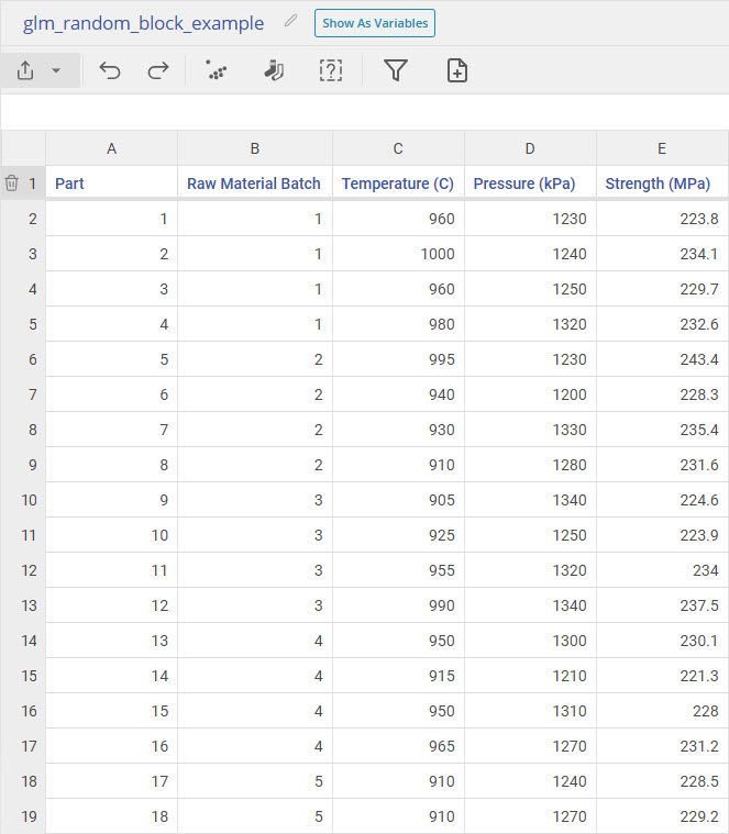
Our first dataset is from a manufacturing process where we are analyzing the effects of Temperature and Pressure on Strength. In our dataset, we have 5 measurements per Raw Material Batch. It is known that strength can vary based on raw material batch, but there is no way to predict exactly what strength the next batch will have, they follow a random distribution.
Let's model strength using temperature and pressure as our independent variables with and without raw material batch as a random effect in the model.
1. Open the General Linear Modeling tool onto the workspace by going to Analyze > Regression Analysis > General Linear Modeling.
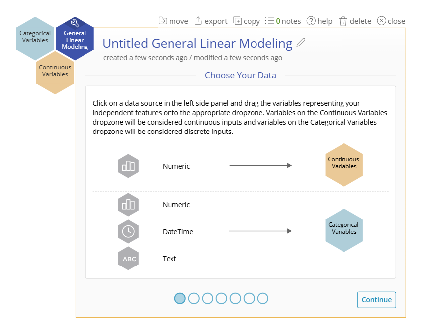
2. Drag Temperature and Pressure onto the Continuous Variables Dropzone, select "Continue", and then drag Strength onto the Response Variable Dropzone.
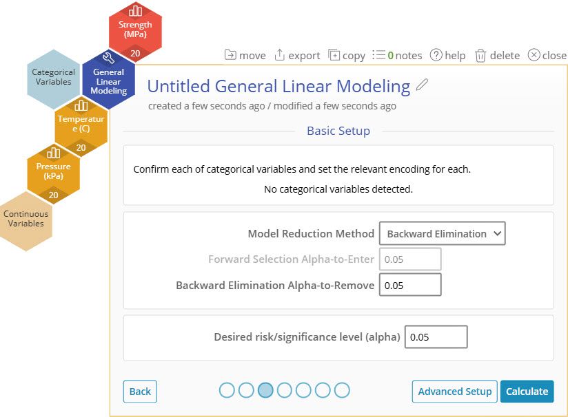
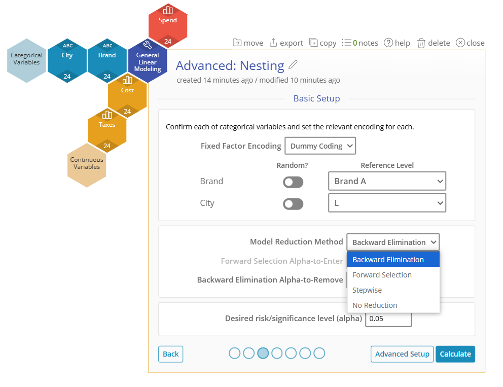
3. One new feature of GLM is the addition of multiple Model Reduction Methods. For this example we will leave on "Backwards Elimination" with an alpha-to-remove of 0.5 as the default.
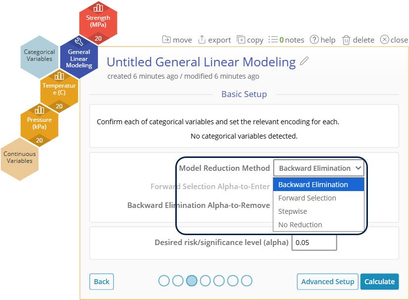
Model Reduction Methods
Note that for all methods, any model terms that are included in a significant higher order term in the model are kept in the model, regardless of their significance, to maintain hierarchy.
Backwards Elimination
- After fitting the model with all terms specified, every model term that has a p-value that exceeds the "Backward Elimination Alpha-to-Remove" is removed from the final model one at a time in the output.
Forward Selection
- Starting with no terms in the model, terms are added one at a time until no more terms with a p-value less than the "Forward Selection Alpha-to-Enter" can be added.
Stepwise
- A combination of forward and backward elimination using both p-value cutoffs to add and remove terms.
No Reduction
- The model specified is fit and no terms are added or removed based on significance.
4. Click "Calculate" to jump straight to the output.
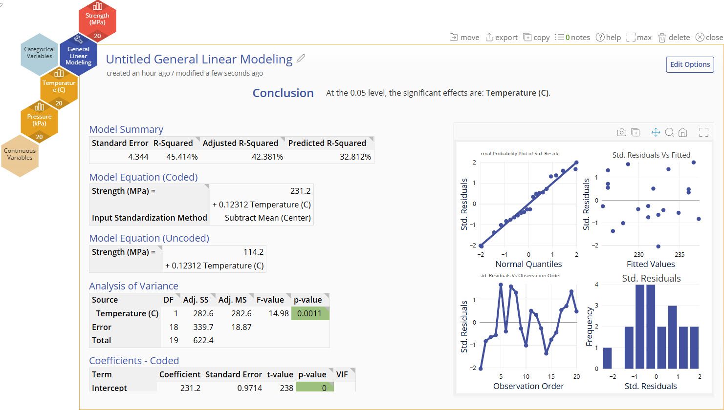
In our output we can see that the model reduction removed Pressure from the model and the model with only Temperature has an R-Squared of 45%. Without including the Raw Material Batch in the model, the batch to batch variation is included in the pure error (noise). This leads to higher p-values for our fixed effect terms and a lower R-Squared.
More information on the model output below.
Fixed Effect Model Output
Conclusion Statement
- Lists which factors are significant at the selected alpha level.
Model Summary
- These statistics help determine whether the model generated is a good fit for your data.
Model Equation (Coded)
- An equation generated using the input standardization method. The default standardization method is Centering, or subtracting the mean. In the Advanced example, we will show how this is set.
- This equation is useful for comparing effect sizes by comparing term coefficients, but this model should not be used for directly predicting the output.
Model Equation (Uncoded)
- An equation generated from your data. Use this model when using real values of your data to predict the output.
Analysis of Variance and Coefficients Tables
- ANOVA table breaking down the significance of the terms in your model. The significant terms are highlighted in green.
Coefficients - Coded
- Coded coefficients of each term, their statistical significance, and their Variance Inflation Factor (VIF)
- VIFs measures how much the given term is correlated with other terms in the model. VIFs greater than 10 typically mean that there is high multicollinearity with other terms in the model and it may be risky to trust the coefficient sizes.
Model Parameters
- Informational table about some of the selected options.
Let's fit the model again with the Raw Material Batch included as a random effect to account for its known random variation.
5. Click "edit options" in the output to go back to "Basic Setup".
6. Drag Raw Material Batch over to the Categorical Variables Dropzone and activate the "Random" slider in the categorical variables setup options.
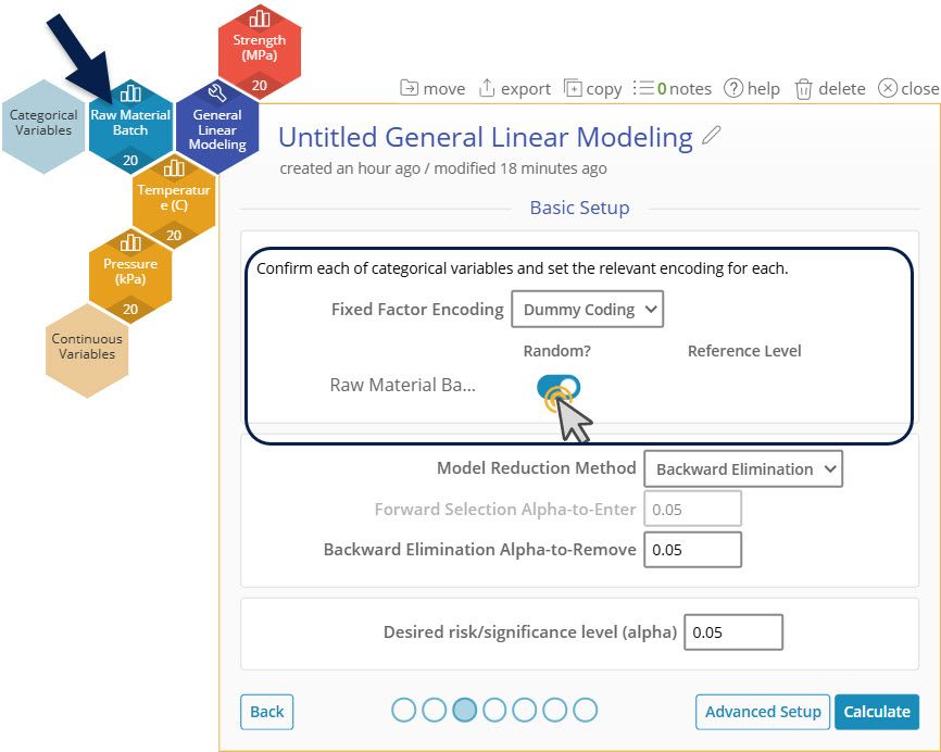
Categorical Variable Setup
First, you have the option here to select which type of encoding you would use. Dummy Coding, also known as One-Hot Encoding, will calculate the coefficients of the categorical levels based on a reference level you select. In Effect Coding, the coefficients of the categorical levels will be set according to the mean. We will leave this at Dummy Coding.
Second, you have the option of setting whether a particular categorical variable is Random. Random variables are variables that are not selected specifically. In this case, our Raw Material Batch number is not something that we are specifically selecting as the Batches will come in randomly and will change in the future as well.
7. Click "Calculate" to jump straight to the output.
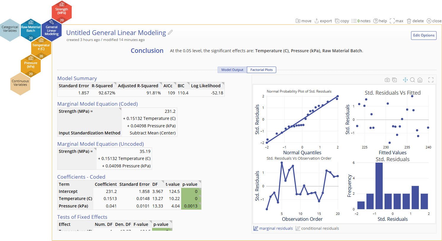
At first glance we see that adding Raw Material Batch as a random block in our model has lead to Pressure being kept in the model and our R-Squared to go from 45% in the last model to 93% now. Accounting for the random batch to batch variation of Strength has lead to a much improved model.
More information on the model output below.
Mixed Model Output
Conclusion Statement
- Lists which factors are significant at the selected alpha level.
Model Summary
- These statistics help determine whether the model generated is a good fit for your data.
Marginal Model Equation (Coded)
- The "Marginal" model does not include the random effect(s) in the model.
- An equation generated using the input standardization method. The default standardization method is Centering, or subtracting the mean. In the Advanced example, we will show how this is set.
- This equation is useful for comparing effect sizes by comparing term coefficients, but this model should not be used for directly predicting the output.
Marginal Model Equation (Uncoded)
- An equation generated from your data. Use this model when using real values of your data to predict the output.
Coefficients - Coded
- Coded coefficients of each term and their statistical significance
- Variance Inflation Factors (VIFs) cannot be calculated in a mixed model
Variance Components
- Breaks down the variation due to pure error (noise) and the random effect(s) in the model. The higher the %Total Variance of the random effect(s), the more significant their p-value.
Model Parameters
- Informational table about some of the selected options.
Random Factors
- Reports the Best Linear Unbiased Predictors (BLUPs) of each level of the given random effect.
- BLUPs are the best guess of the effect of each level of the random effect.
Conditional Model Equation (Coded)
- Unlike the "Marginal" model, the "Conditional" model does include the random effect(s) in the coded model.
Example 2 (Interactions and Higher Order Terms)
This dataset contains Activity and Weight as input variables and Bone Density as a response variable.
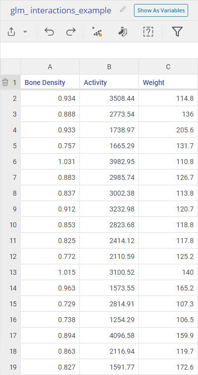
1. Open the General Linear Modeling tool onto the workspace by going to Analyze > Regression Analysis > General Linear Modeling.
2. Click on the Data Source and drag on Activity variable and the Weight variable onto the Continuous Variables Dropzone.
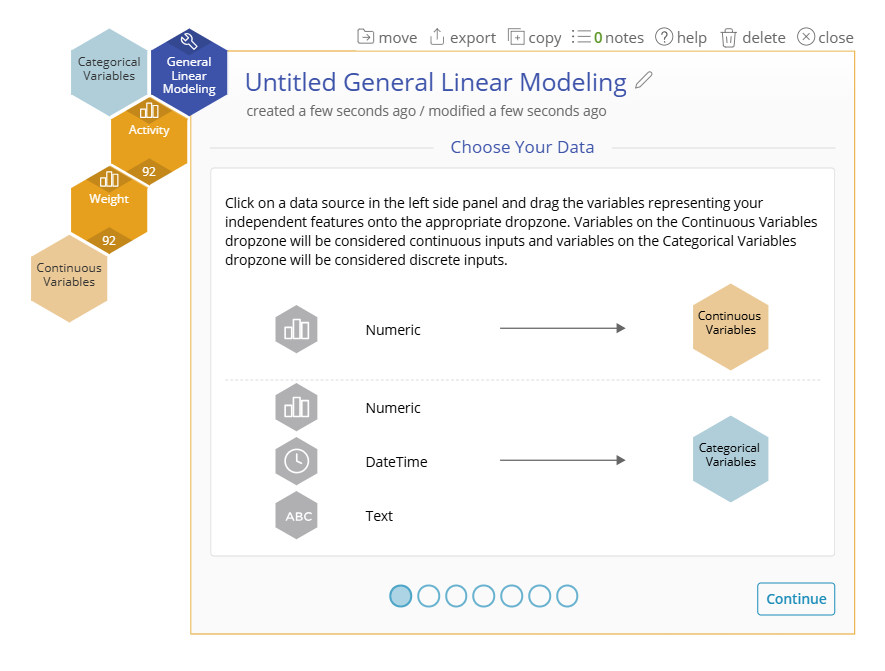
3. Click Continue.
4. Drag on the Bone Density variable onto the Response Variable Dropzone.
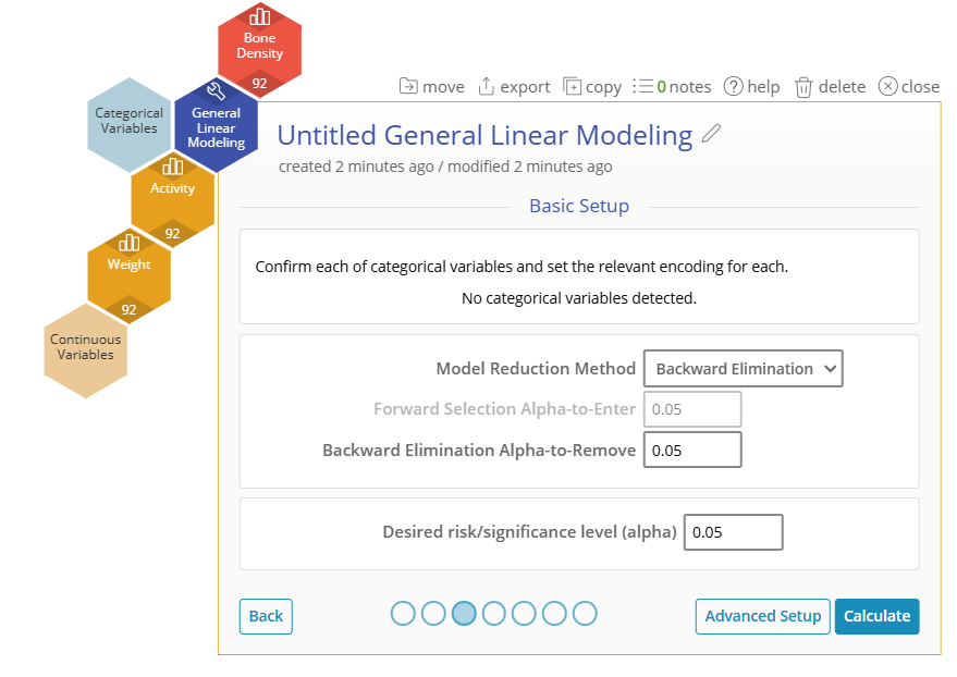
5. We are going to leave the Basic Setup options at their defaults.
6. Click on Advanced Setup.
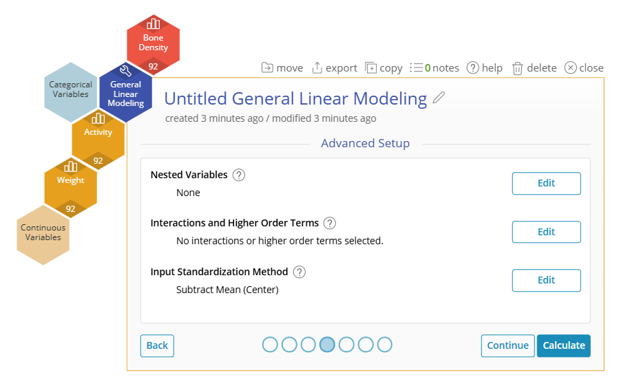
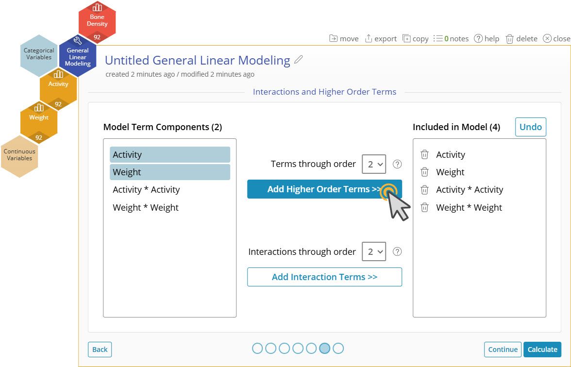
7. Click on the "Edit" button next to "Interactions and Higher Order Terms". The Interactions and Higher Order Terms screen allows you to select which interactions or higher order terms you want to consider for the model. This adds additional complexity to your model, so be aware when adding many interactions or higher order terms.
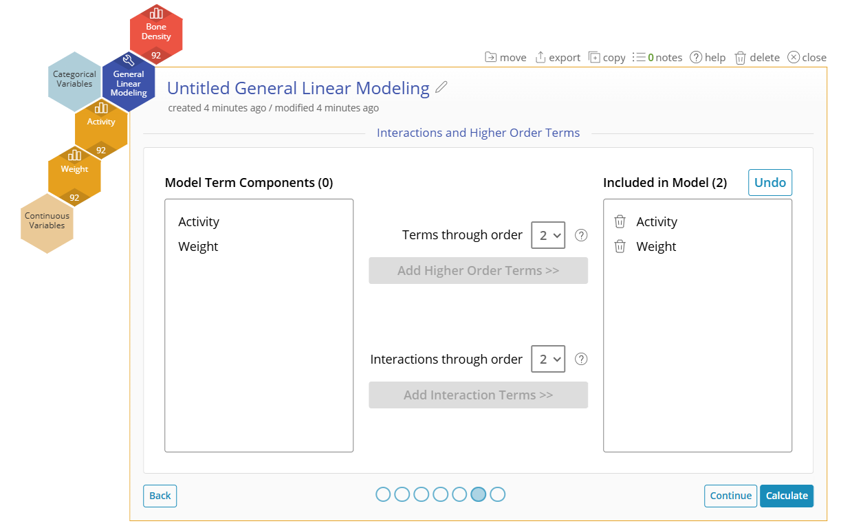
8. Click on both Activity and Weight on the left side.
9. Click on "Add Higher Order Terms >>" to add the quadratic terms Activity * Activity and Weight * Weight to the model.
11. Click "Add Interaction Terms >>" with Activity and Weight still selected on the left. This will add Activity * Weight to the model.
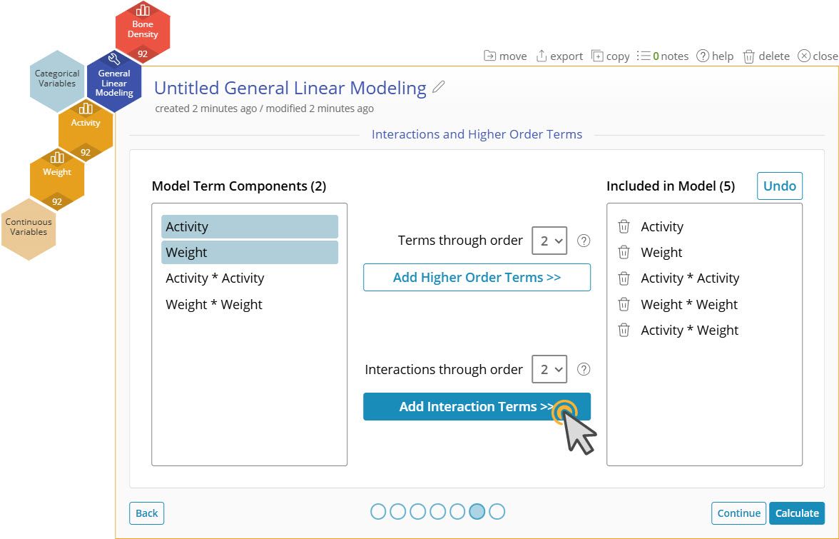
Note : Adjusting the number in the dropdown allows you to add 3rd order terms and three-way interactions.
12. Click "Calculate".
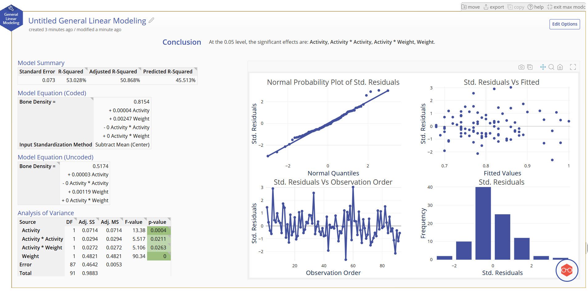
Our model shows a moderate fit to the data and removed the Weight quadratic term (Weight * Weight) in the model reduction phase. We expected a large amount of noise in this response variable, so seeing these terms as significant including is a success in learning how our factors can impact our response.
More information on the model output below.
Fixed Effect Model Output
Conclusion Statement
- Lists which factors are significant at the selected alpha level.
Model Summary
- These statistics help determine whether the model generated is a good fit for your data.
Model Equation (Coded)
- An equation generated using the input standardization method. The default standardization method is Centering, or subtracting the mean. In the Advanced example, we will show how this is set.
- This equation is useful for comparing effect sizes by comparing term coefficients, but this model should not be used for directly predicting the output.
Model Equation (Uncoded)
- An equation generated from your data. Use this model when using real values of your data to predict the output.
Analysis of Variance and Coefficients Tables
- ANOVA table breaking down the significance of the terms in your model. The significant terms are highlighted in green.
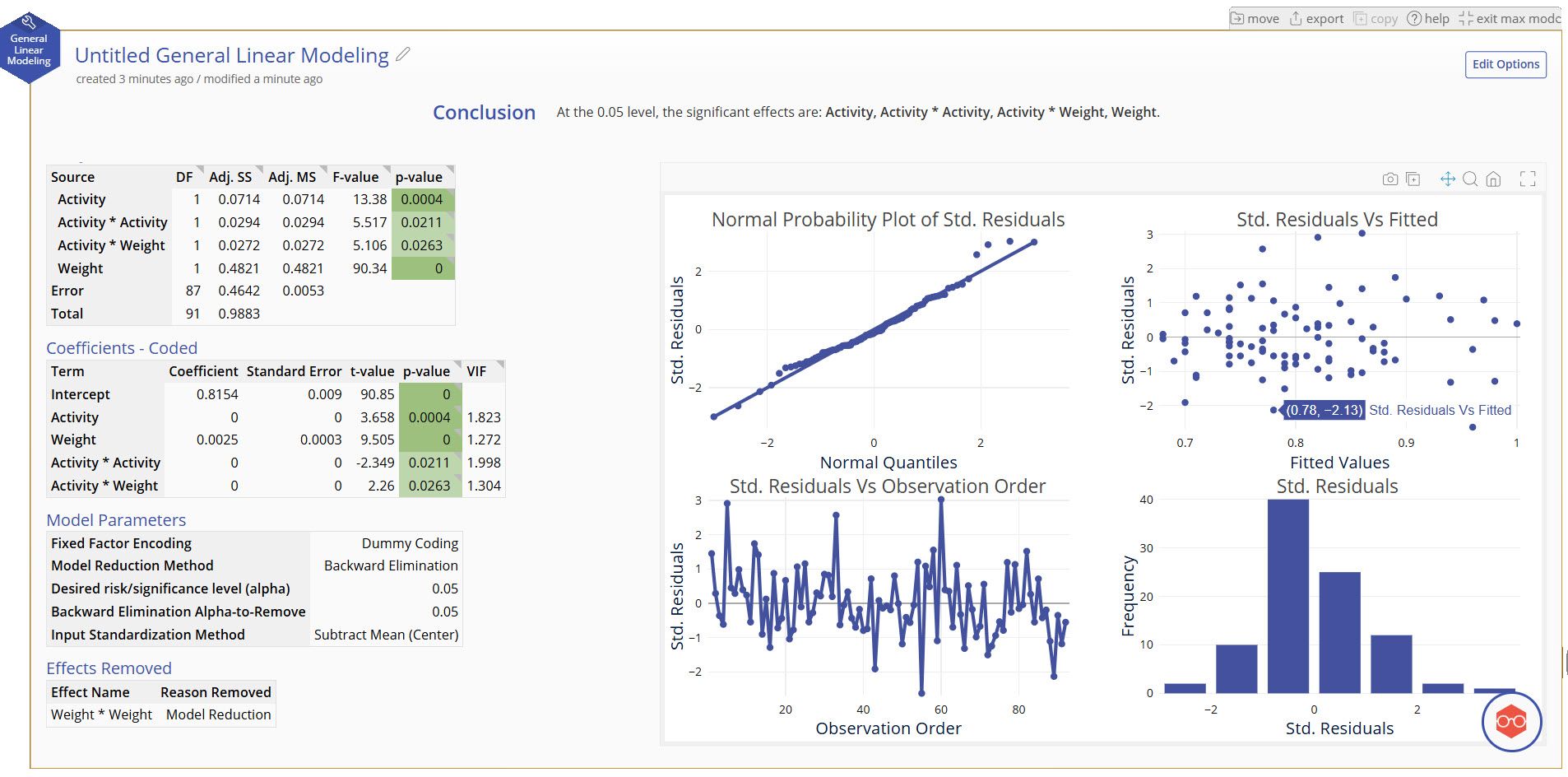
Coefficients - Coded
- Coded coefficients of each term, their statistical significance, and their Variance Inflation Factor (VIF)
- VIFs measures how much the given term is correlated with other terms in the model. VIFs greater than 10 typically mean that there is high multicollinearity with other terms in the model and it may be risky to trust the coefficient sizes.
Model Parameters
- Informational table about some of the selected options.
Example 3 (Nested Terms)
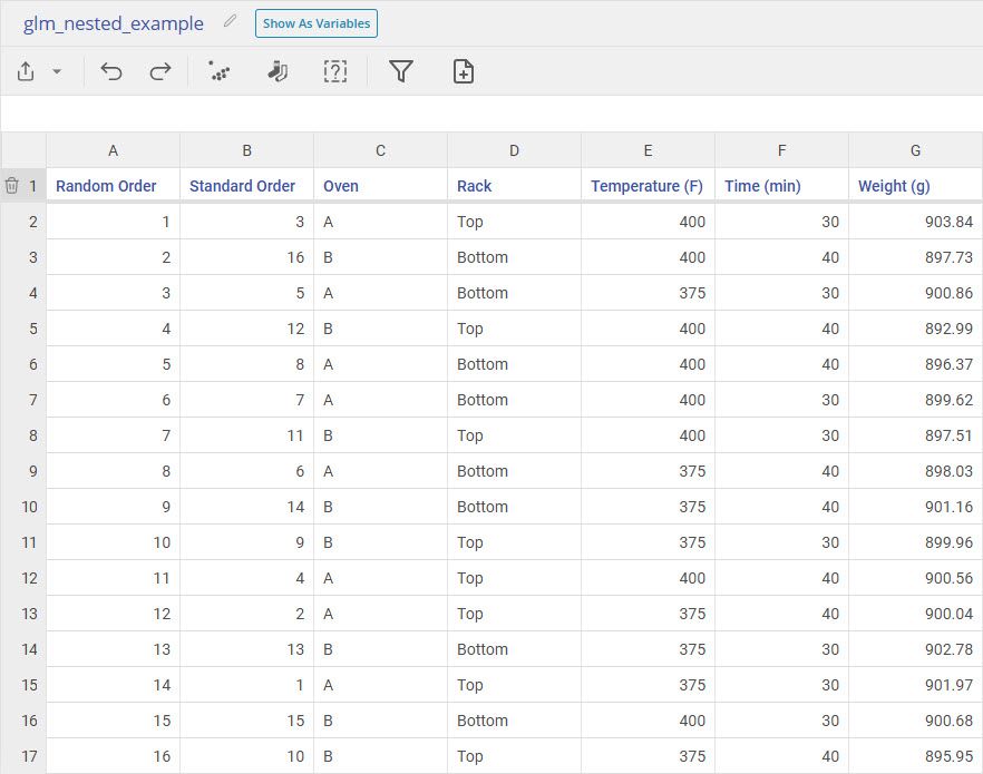
The baking company "Rise and Shine" wants to find the optimal Time and Temperature to bake their bread at in order to get the optimal loaf Weight of 900 grams. They have two bread baking Ovens, each with its own unique top and bottom Rack positions. Because the racks are physically different from one oven to another, the bakers consider Rack to be nested within Oven.
To study the effects of Time and Temperature while accounting for variation between ovens and racks, the bakers ran a designed experiment varying Time and Temperature across the two ovens, with measurements taken from each Rack within each Oven. The results from this completely randomized experiment are shown below.
Nested Terms are used when the levels of one of the factors in your model is part or reliant upon the levels of another factor. In this example, which rack the bread is baked on depends on both the oven and the rack (e.g. the top rack of oven A is not the same as the top rack of oven B). Thus we say that "rack is nested in oven".
1. To start, open the General Linear Modeling tool onto the workspace by going to Analyze > Regression Analysis > General Linear Modeling.
2. Click on the Data Source then drag the variables Oven and Rack onto the Categorical Variables Dropzone. Drag the variables Temperature (F) and Time (min) onto the Continuous Variable Dropzone.
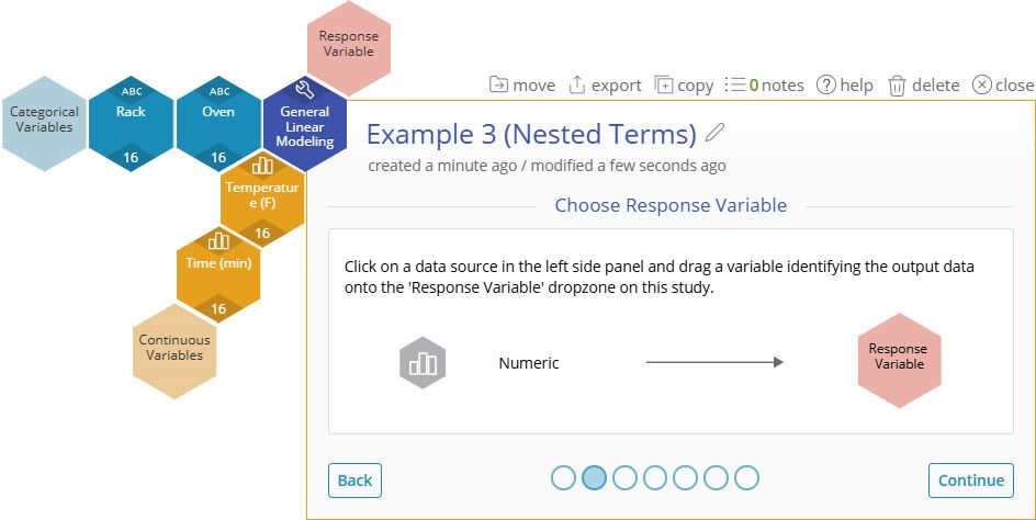
3. Drag on the variable Weight (g) onto the Response Variable Dropzone.
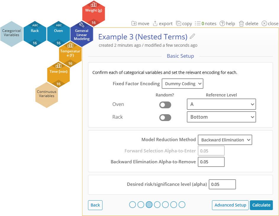
4. Leave the Basic Setup options as they are, and click on "Advanced Setup."
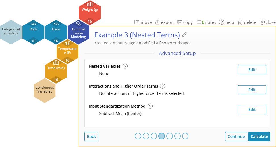
5. On the Advanced Setup screen, click "Edit" for Nested Variables.
6. On the Nested Variables screen, select Rack is nested in Oven.
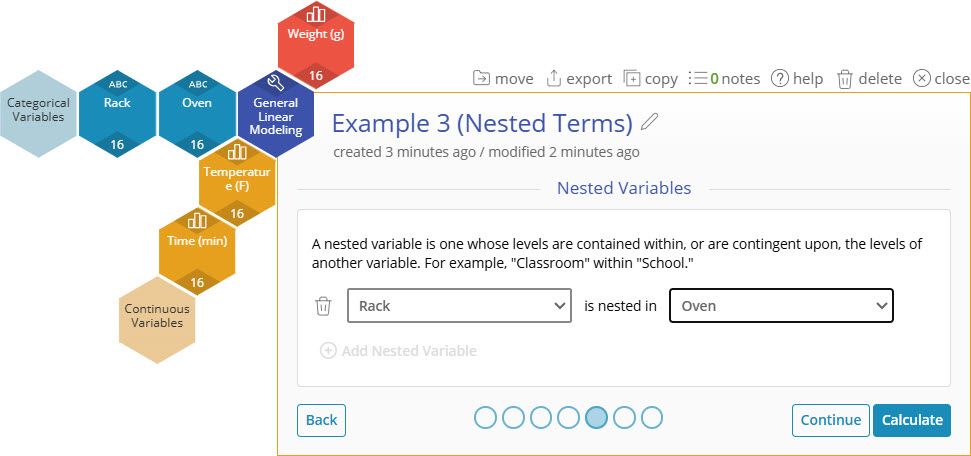
7. Click "Calculate".
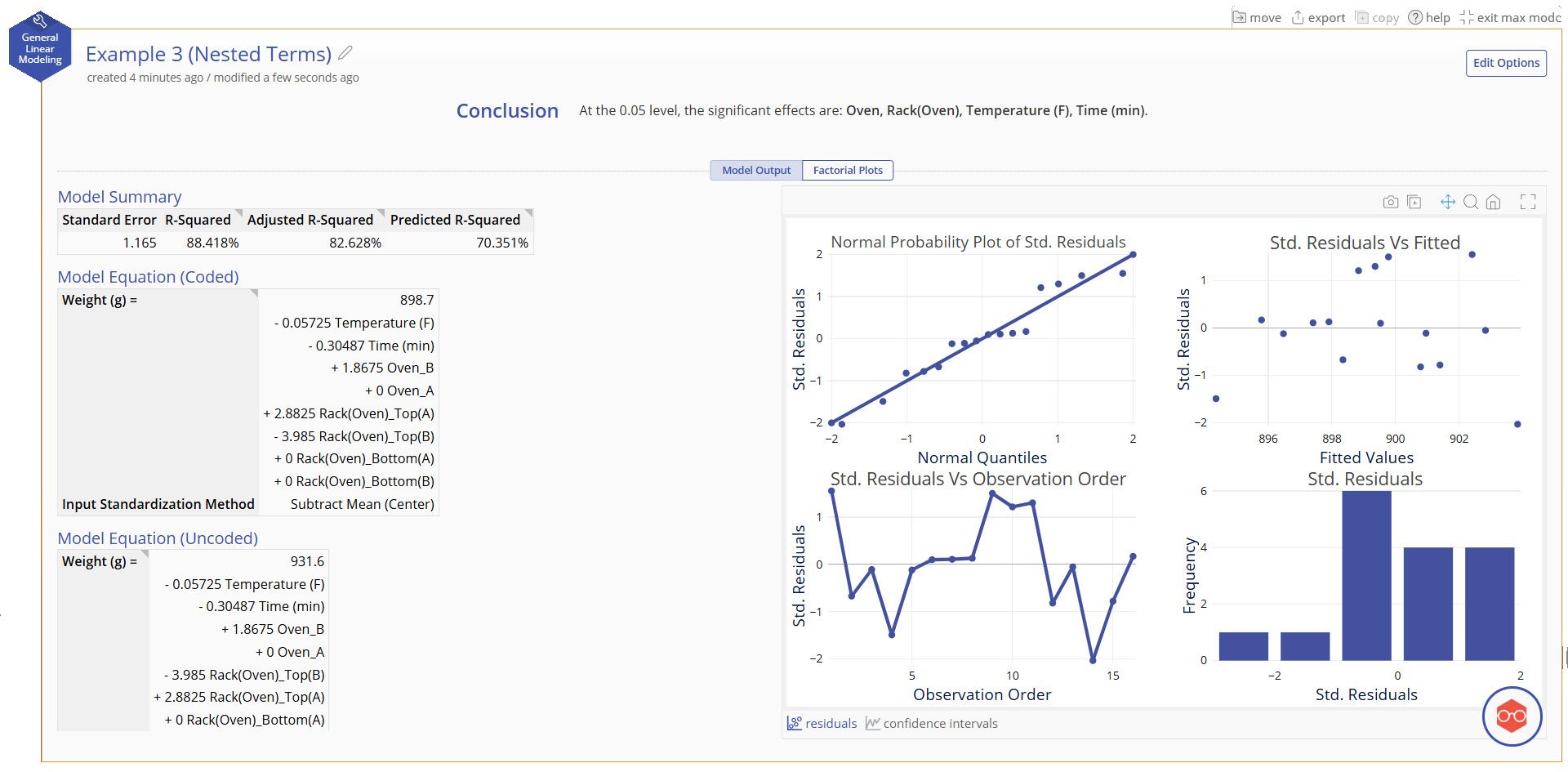
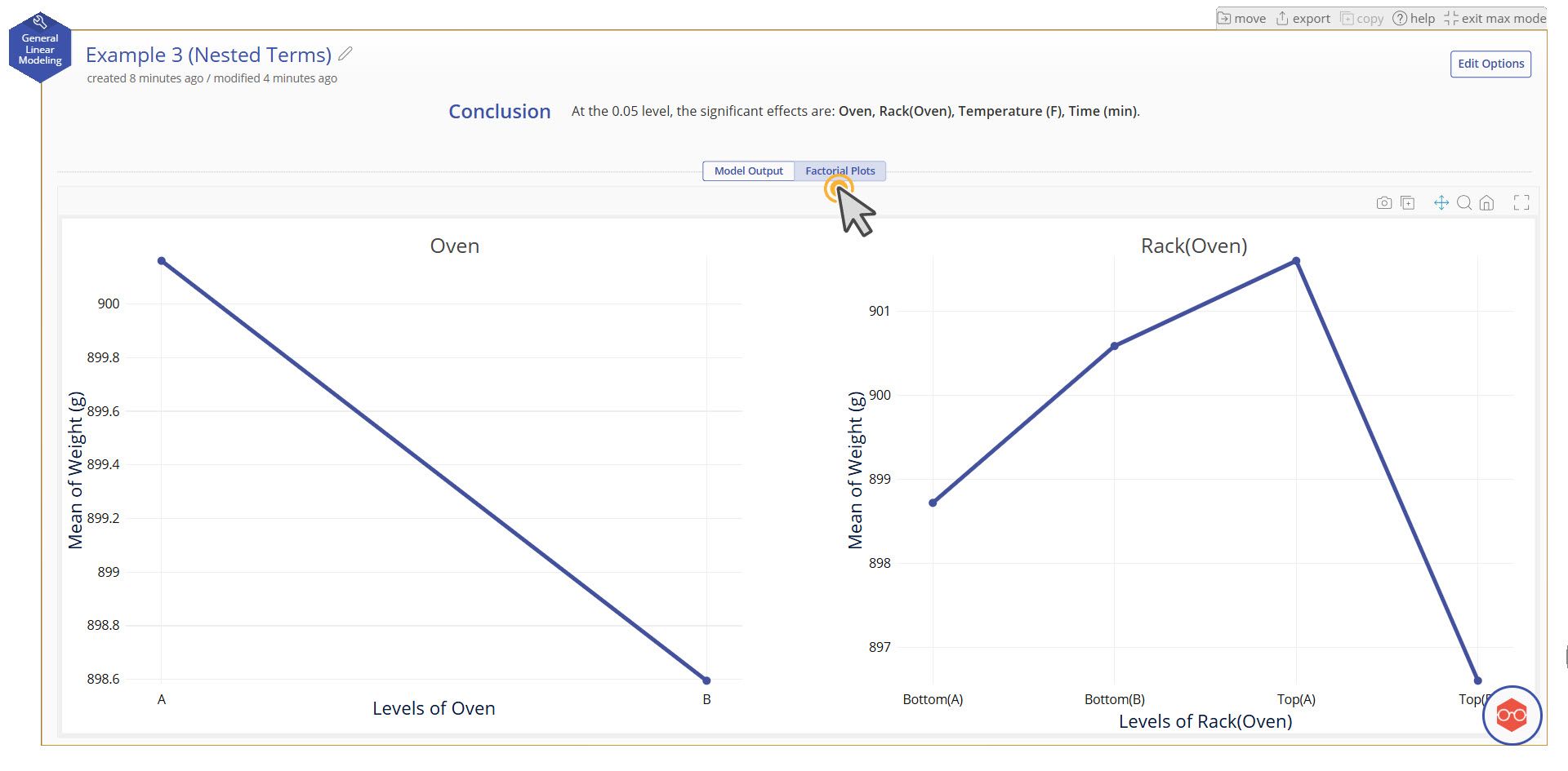
Our model shows good fit to the data and includes all model terms. Notice that the term for Rack is "Rack(Oven)". This is the parentheses nomenclature to represent Rack being nested in Oven.
We can interpret the model similarly to how we have in the previous examples. The "Tukey Adjustment" table for differences in our categoric variables and the "Factorial Plots" are new focuses of this output.
More information on the model output below.
Fixed Effect Model Output (with Categorical Variables)
Conclusion Statement
- Lists which factors are significant at the selected alpha level.
Model Summary
- These statistics help determine whether the model generated is a good fit for your data.
Model Equation (Coded)
- An equation generated using the input standardization method. The default standardization method is Centering, or subtracting the mean. In the Advanced example, we will show how this is set.
- This equation is useful for comparing effect sizes by comparing term coefficients, but this model should not be used for directly predicting the output.
Model Equation (Uncoded)
- An equation generated from your data. Use this model when using real values of your data to predict the output.
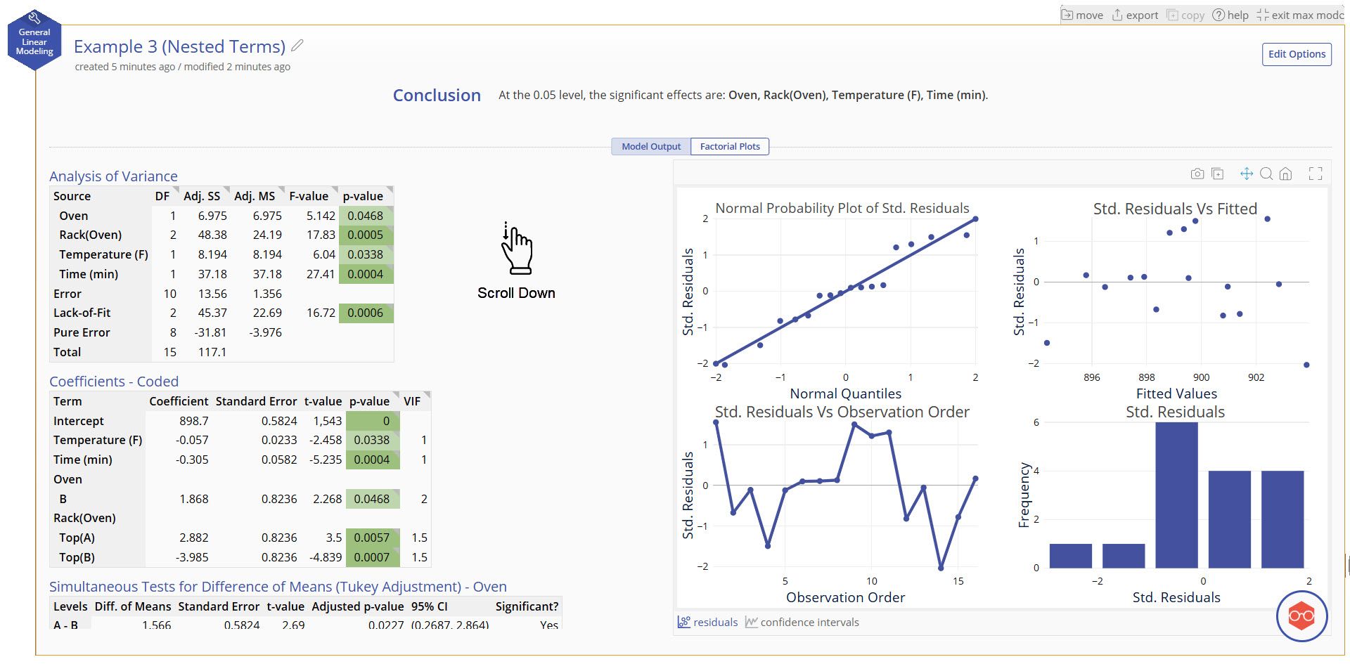
Analysis of Variance and Coefficients Tables
- ANOVA table breaking down the significance of the terms in your model. The significant terms are highlighted in green.
Coefficients - Coded
- Coded coefficients of each term, their statistical significance, and their Variance Inflation Factor (VIF)
- VIFs measures how much the given term is correlated with other terms in the model. VIFs greater than 10 typically mean that there is high multicollinearity with other terms in the model and it may be risky to trust the coefficient sizes.
Model Parameters
- Informational table about some of the selected options.
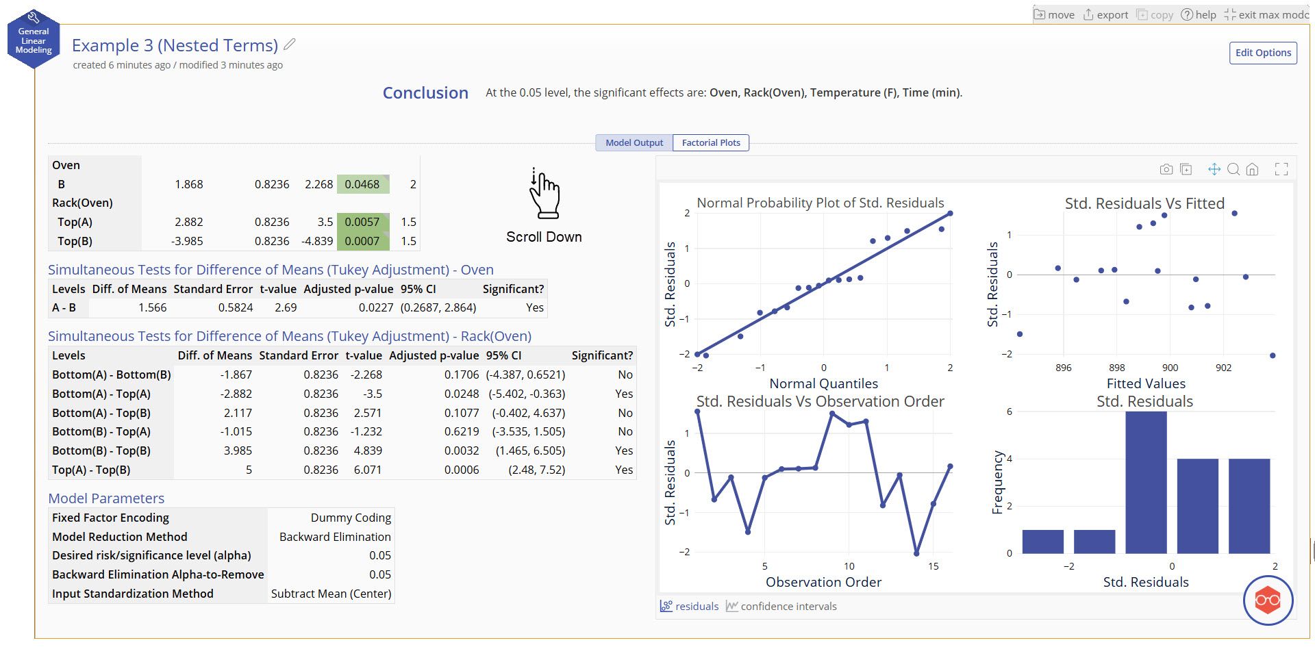
Simultaneous Tests for Difference of Means (Tukey Adjustment)
- For each categorical variable in the model, this table tests the statistical significance of all paired differences between every combination of levels in the variable.
- The confidence interval and p-value can both be used to assess significance.
- The "Confidence Intervals" plots in the bottom right of the output visualize these differences and confidence intervals.
Note also that there are two tabs at the top. Switching to the tab called "Factorial Plots" will show the main effect plots for the categorical variables in the model. Here we can see the average difference between ovens A and B, as well as see the differences between the 4 unique racks.
Additional Options
Two other options not previously discussed:
Basic Setup Screen:
Model Reduction Method: Used to simplify the model by adding or removing factors based on their significance. Choose from Backward Elimination, Forward Selection, Stepwise, or No Reduction.
Advanced Setup Screen:
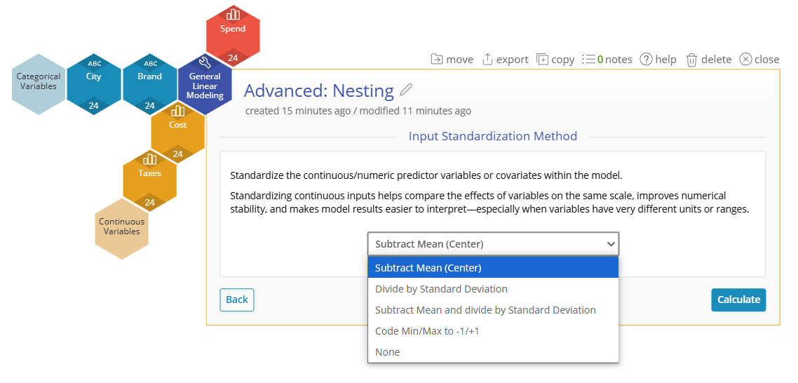
Input Standardization Method: Sets how you might be interested in comparing coefficients on the same scale. The options are Subtract Mean (Center), Divide by Standard Deviation, Subtract Mean and Divide by Standard Deviation, Code Min/Max to -1/+1, or None.
Was this helpful?