Hypothesis Testing Wizard

The Hypothesis Testing Wizard offers you different options to select a test to analyze your data. If you are new to hypothesis testing use the Question and Answer mode; if you're an experienced user you can directly select the exact test of your choice from one of the Test Maps available.

As you draw your conclusions, keep in mind that inferences from hypothesis tests apply to the data sampled at a particular point in time. If you want to assess a population characteristic over time, consider using a Trend Chart or Control Chart instead.

In the Contents menu to the left, go to Tools > Hypothesis Testing > Hypothesis Testing Wizard to see all the topics associated with the Wizard.

Wizard Mode

The Wizard is a responsive and dynamic tool that leads you through a series of questions and automatic validations to select an appropriate test for the data at hand.

Hypothesis Testing Wizard:

The basic flow goes through five steps:

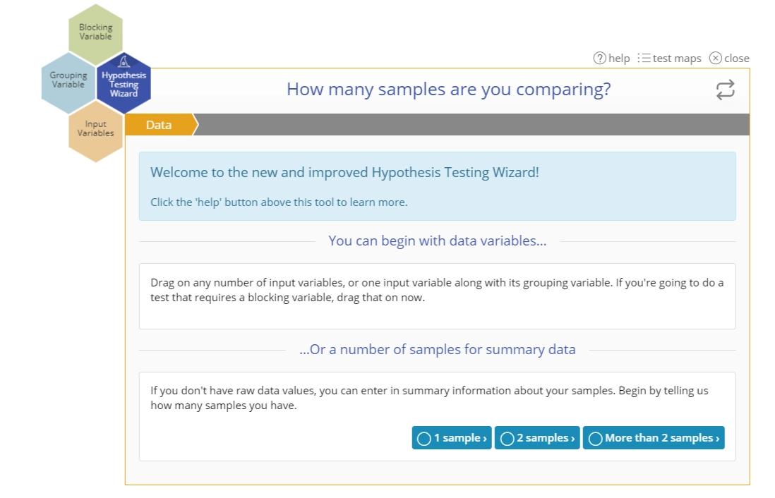
1. Data: In this step you can either drag on your variable(s), or if you have summary data, select the number of samples you want to compare.
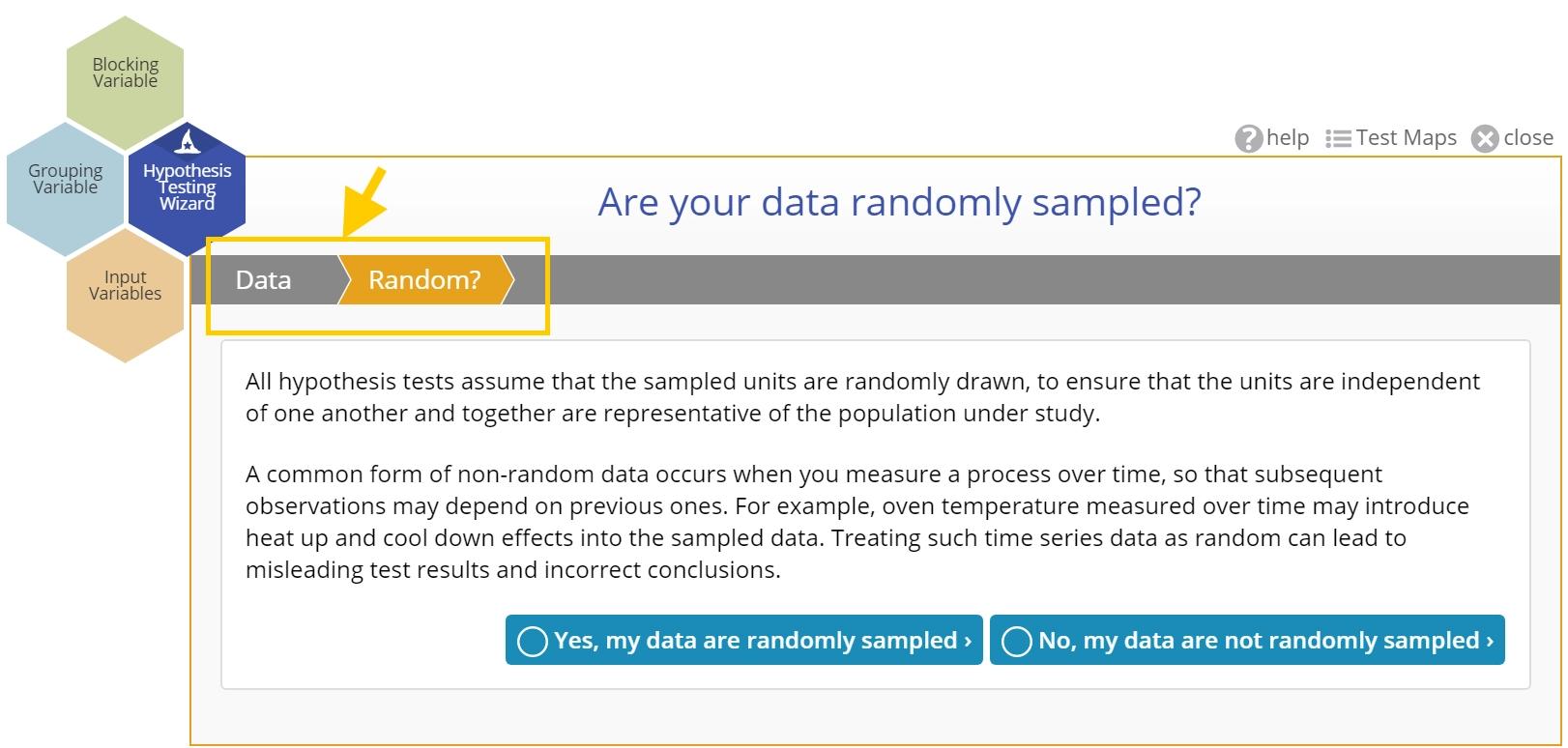
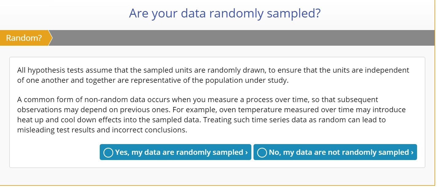
2. Random?: Here you have to answer the question, "Are your data randomly sampled?". Randomly drawn data is a key assumption underlying all hypothesis tests.
3. Objective: In this step you will select the parameter about which you wish to test a claim from among four possible options: Proportion, Mean, Median, or Variance. Note: based on your previous selections, some parameters may not be available for selection; for example, if you have dragged on continuous data variables, the 'Proportion' option will not be available because it only applies to binary data.
4. Assumptions: The wizard automatically checks the assumptions relevant to the potential tests associated with the chosen parameter and the data, if present. Read the evaluations so you understand the requirements of the test and note any assumption violations which may lead to a different test than expected.
5. Construct: Once you accept the test assumptions, you can construct the test by entering information which helps set up the null and alternative hypotheses and other test requirements.

Notes:

1. If you drag on data variables in step 1 (instead of selecting the number of samples for summary data entry), the step 1 screen disappears and the process starts at step 2: Random?. If you're using the summary data option, the step 1 screen persists to allow you to change the number of samples selected.
2. Some tests, such as the Proportion tests, have a larger number of steps because they have more assumptions that must be validated. Others have fewer steps due to fewer assumptions.

When the setup is complete, click the button to launch the recommended test. A separate, standalone study opens in which the test results are displayed along with the evaluated assumptions and output graphs.

If you have an objective and a fairly good idea of the test to use, but are unsure of the most appropriate test or the requirements for the test, you can use the 'Test Maps' mode to quickly identify the appropriate test (go to the next help article for more information).

Test Maps Mode

Use the 'Test Maps' mode to quickly identify the most appropriate test for your desired objective and available data. There are two test maps - Parametric and Non-Parametric. Each map shows a decision tree of the conditions/assumptions leading to the recommended test.

The two test maps are shown below:

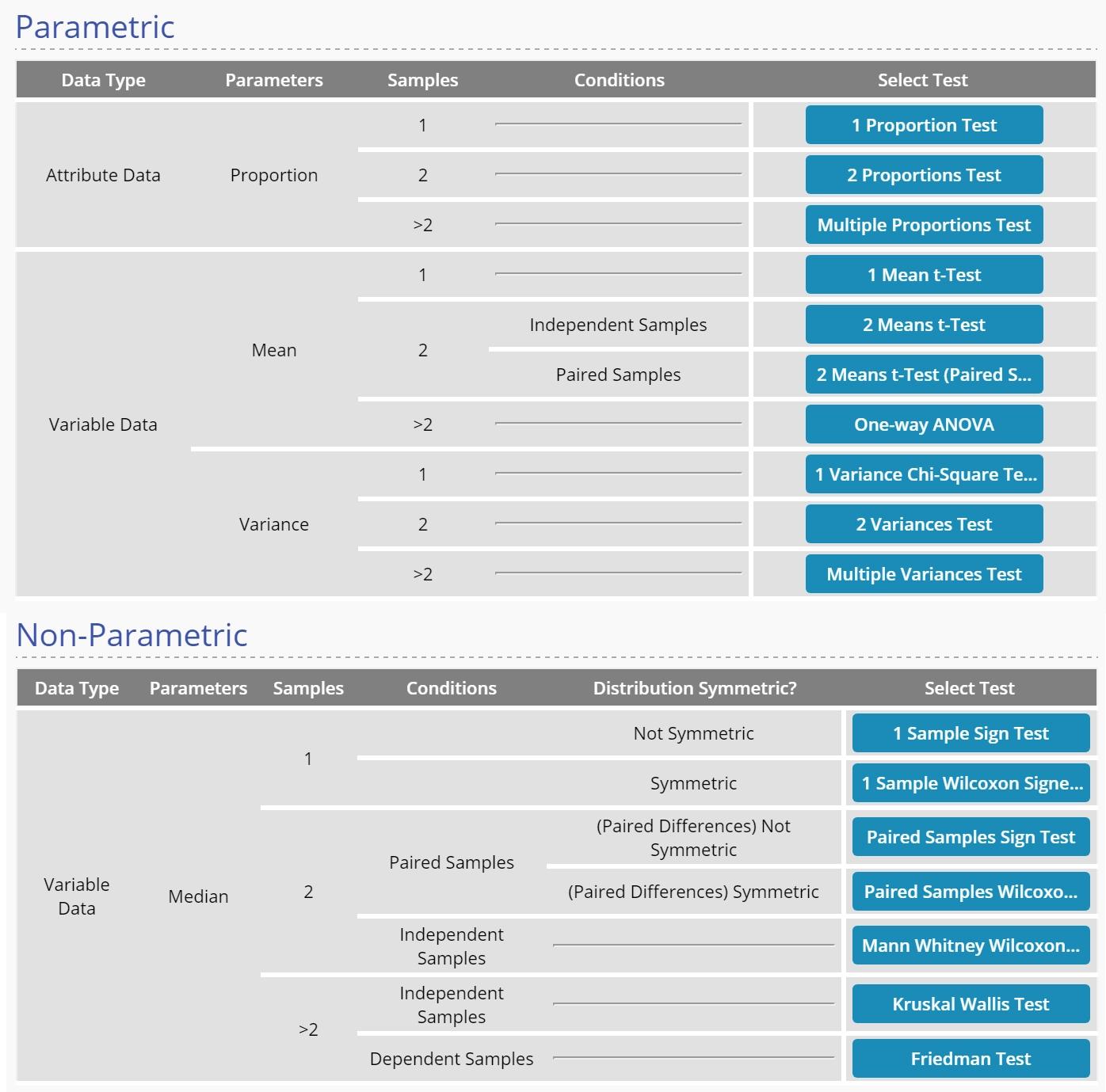
Selecting a test from the test map opens a standalone hypothesis test study. Here you can enter information in the Settings panel and drag on data variables or select the Summary Data tab to enter summary data. To read about how to run the test in the standalone study, go to the article under: Tools > Hypothesis Testing Standalone Tests.

Select Data

This is the first step in the Hypothesis Testing Wizard mode. If you have raw data (columns of data in a data source), you can drag the variables on to the appropriate drop zones on the Wizard. If you don't have raw data, you can select the number of samples for which you would like to input summary statistics.

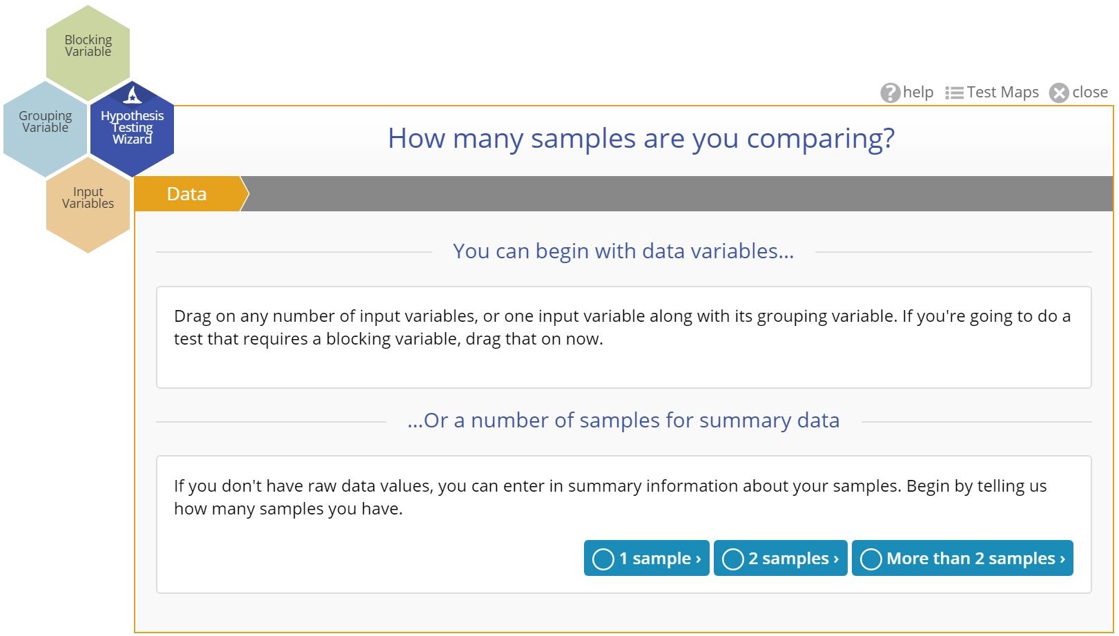
If you drag on one or more data variables, the wizard will skip this step and ask you to confirm the data are random:

If you instead select the number of samples for summary data input, the wizard will show step 2 and ask you to confirm the data are random:

This is because once you identify the data you do not need to come back to this step - you can always change the number of data variables chosen by dragging them on or off the wizard. For summary data on the other hand, you'd need to return to this step to change the number of samples.

Are Your Data Randomly Sampled?

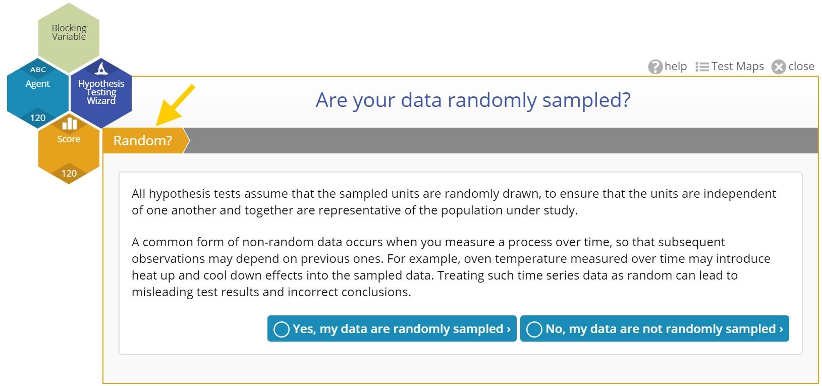
Hypothesis tests assume that the data samples are randomly drawn, to ensure that individual observations are independent of each other and that the observations are not correlated across time or any other factor.

In the wizard, this is step 2 of the test flow:

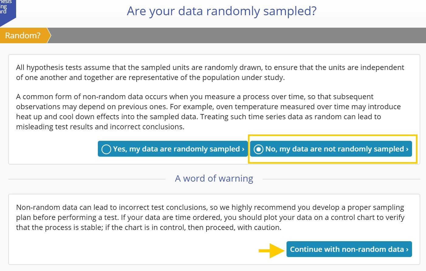
If you indicate Yes, the wizard will move on the the next step. If you indicate No, it will warn you about the negative consequences of using non-random data for hypothesis testing, but give you the option to proceed regardless:

Why do you need random data?

If the observations are not selected in a random manner, you run the risk of getting a sample that is not truly representative of the population under study, rendering the test results meaningless.

To draw a random sample, number all the units in the population and use a table or software that generates random numbers to pick the units corresponding to those numbers, and include those units in the sample. Obviously, this isn’t always practical or even possible, but that doesn’t mean that you cannot use hypothesis testing.

Let's say a hospital measures patient registration wait times over a month. As long as the wait times are measured at randomly selected times of day throughout the week, the sample can be considered to be random. But if the wait times are measured at the same time each day, or only every Saturday, there is a high chance the data are not independent or representative of the actual wait time process. In that case, your data may not tell you anything of value about the process. If you have time-ordered data of this type, it is recommended that you plot your data on a Trend Chart or Control Chart instead. If the process is stable and the data are within control, you may be justified in taking the hypothesis testing approach, with care.

Select Test Objective

In the third step in the Hypothesis Testing Wizard Q/A mode (second if you drag on variables), you are prompted to indicate what it is you wish to test or compare:

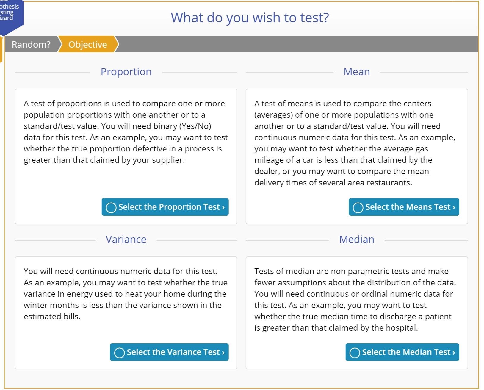
Options:

Proportion

The proportion is the relative number of specified events in a set of data, where the event is one of only two possible outcomes for each data observation. It is calculated as the number of occurrences of the specified event divided by the total number of observations in the set.

A test of proportions is used to compare one or more population proportions with one another or to a standard/test value. You will need binary (Yes/No) data for this test. As an example, you may want to test whether the true proportion defective in a process is greater than that claimed by your supplier.

Mean

The mean or average is a summary value that explains the centering of a set of data. If your data are skewed, then the mean will not correctly represent the true center of the data – in this case it is better to use the median.

A test of means is used to compare the centers (averages) of one or more populations with one another or to a standard/test value. You will need continuous numeric data for this test. As an example, you may want to test whether the average gas mileage of a car is less than that claimed by the dealer, or you may want to compare the mean delivery times of several area restaurants.

Median

If you have an odd number observations in your sample, the median is the middle-most value in the data set. If you have an even number observations in your sample, the median is the average of the two middle-most values in the data set.

A test of medians is used to compare the centers (medians) of one or more populations with one another or to a standard/test value. This test is usually performed when the corresponding parametric test of the mean is not recommended due to violation of the assumption requiring normal distribution of variables. Tests of median are non-parametric tests which make fewer assumptions about the distribution of the data. You will need continuous or ordinal numeric data for this test. As an example, you may want to test whether the true median time to discharge a patient is greater than that claimed by the hospital.

Variance

The variance is a measure of the spread or range of the data set. It is calculated as the average squared distance of each observation in the data set from the mean of the data set.

A test of variances is used to compare one or more population variances with one another or to a standard/test value. You can use this test to check the assumption of equal variances required by some tests of means and medians. You will need continuous numeric data for this test. As an example, you may want to test whether the true variance in energy used to heat your home during the winter months is smaller than the variance shown in the estimated bills.

Checking the Test Assumptions

Every test, whether parametric or non-parametric, is based on a certain set of assumptions. Non-parametric tests make fewer and weaker assumptions than their parametric counterparts, but they still make assumptions. Checking these assumptions ensures the validity of the test for the data at hand.

For example, you may have a sample of data on which you want to carry out a proportions test. All the available proportions tests make the assumption that the probability of the event of interest is constant across all population (and therefore across all sample) units. If this is not true, the units will have different underlying chance of having the event occur and they're no longer comparable. Any results of a test run on these data would be inaccurate and could lead to the wrong decisions. So it is important to assess the assumptions for any violations and either take mitigating action or use a more robust test.

The Wizard checks the assumptions using standard methods and tests and has inbuilt mitigating rules for when a violation is not serious enough to abandon the test.

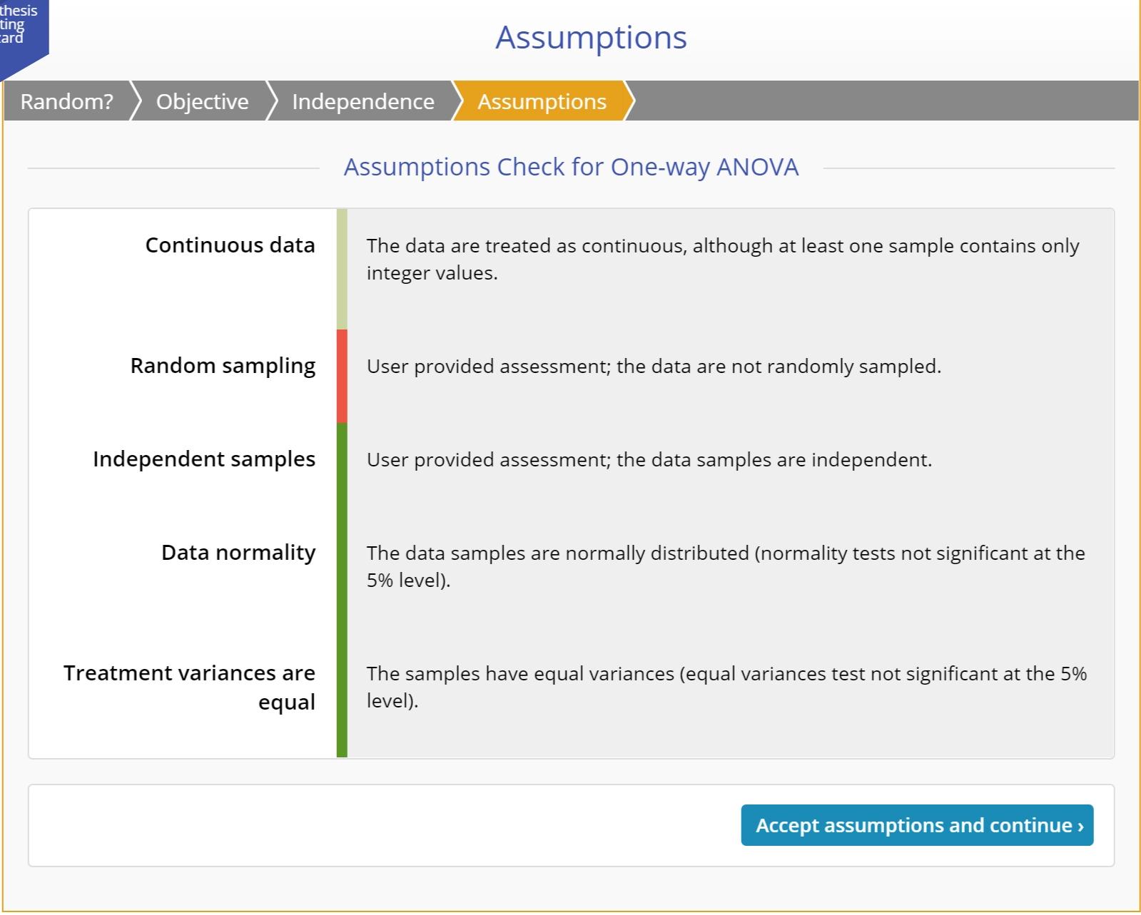
Assumptions:

Here's a list assumptions made by tests of the various parameters:

Proportion

1. The data are binary – each variable consists of two unique values (e.g.: Pass/Fail).
2. The data are randomly sampled.
3. The probability of occurrence of the event is constant across all units.
4. (For two or more samples): The data samples are independent of each other.

Mean

1. The data are continuous.
2. The data are randomly sampled.
3. The data are normally distributed.
4. (For two or more samples on different subjects): The data samples are independent of each other.
5. (For two or more samples on the same subjects): The data samples are paired/dependent.
6. (For paired samples) The paired differences are normally distributed.
7. (For independent samples) The data variables have equal variances. If this assumption is violated, the Wizard automatically directs you to the Unequal-variances t-Test.
8. (For a multiple sample ANOVA test with a blocking variable): The block variances are NOT equal.
9. (For a multiple sample ANOVA test with a blocking variable): The treatments and blocks do not interact with each other.

Median

1. The data are continuous.
2. The data are randomly sampled.
3. (For a Sign Test): The data variable is NOT symmetric.
4. (For a Wilcoxon Signed Ranks Test): The data variable is symmetric.
5. (For a Paired samples Sign Test): The distribution of paired differences is NOT symmetric.
6. (For a Paired samples Wilcoxon Signed Ranks Test): The distribution of paired differences is symmetric.
7. (For a Mann Whitney Wilcoxon or Kruskal-Wallis Test): The data samples are independent of each other.
8. (For a Mann Whitney Wilcoxon or Kruskal-Wallis Test): The data variables have equal variances.
9. (For a Friedman Test): The block variances are equal.
10. (For a Friedman Test): The treatments and blocks do not interact with each other.

Variance

1. The data are continuous.
2. The data are randomly sampled.
3. The data are normally distributed.
4. (For two or more samples): The data samples are independent of each other.

Test Setup

This is the final step in the Hypothesis Testing Wizard Question/Answer mode. Once you have made your selections in the prior steps, the wizard will identify the most appropriate test and bring you to this step which provides a dialog to specify the setup and criteria for the test decision.

The test setup screen typically includes:

• Significance level (alpha)
• Test standard
• Direction of the Alternative hypothesis (Not equal to/Greater than/Less than)
• Any other items specific to the test

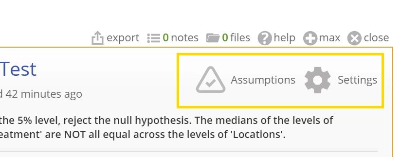
After filling out the test setup screen, you can click the 'Launch test' button which opens the test in a standalone study along with the test output and recommended decision. The output includes two buttons at the top-right: One for the Assumptions assessments made previously and a 'Settings' option to change any of the test setup inputs on the fly without having to go through the entire Wizard over again.

Significance Level (alpha)

Whenever you run a test, there is always a chance that you will get a significant result purely by chance. The Significance Level or alpha is the amount of risk you’re prepared to take of getting such a false positive result (that is, of rejecting the null hypothesis when in fact the null hypothesis is true). It is expressed as a proportion or percentage and represents what proportion, out of a very large number of samples of the same size, is likely to return a false positive result.

Traditionally, values of alpha are set to 1% (0.01), 5% (0.05) or 10% (0.10), although you may enter any value greater than 0 and less than 1, keeping in mind that you want to keep the false positive rate as low as possible, while still allowing the test to detect an effect. By default, EngineRoom sets the value of alpha at 0.05. The default significance level of 0.05 means that if you performed the test on 100 samples of the same size, about 5 of them will incorrectly reject the null hypothesis, i.e., you have a 5% rate of false positives.

The complement of the significance level, (1-alpha), is called the confidence level.

Test Standard/Reference Value

The Test Standard or Reference Value is the value of the parameter (this could be a proportion, mean, median, or variance or it could be the difference of two proportions/means/medians or the ratio of two variances) that you will assume to be true under the null hypothesis. It often represents the historical or status-quo situation that you wish to disprove using the data.

As an example, in a one proportion test you may want to test a supplier’s claim that the true proportion defective in their product is 0.01. In this case, '0.01' is the test standard or null hypothesis value. If your test fails to reject the null hypothesis, then you will continue with the belief that the supplier’s claim is true.

Cut-off Values

Cut-off or critical value(s) for a hypothesis test are values from the reference distribution corresponding to the chosen significance level and the sign of the alternative hypothesis, which is/are compared to the test statistic in order to determine whether or not to reject the null hypothesis. Cut-off values define the rejection region (also called critical region) for the null hypothesis.

p-Value

The p-value is the probability that the model output is the result of pure chance rather than an actual relationship between variables. A p-value which is less than the alpha level selected indicates that the model falls within the accepted risk level. The results are deemed to be "statistically significant" at the chosen significance level.

Confidence Intervals

A Confidence Interval gives a range of possible values of the characteristic of interest (proportion, mean, variance, difference of proportions or means, ratio of variances) that may occur at a given confidence level. It is calculated as a best estimate plus or minus a "margin of error". For example, a national political poll may report a job approval rating for the president as 60% +/- 2.5%, at a 95% confidence level. From those statistics we can conclude with 95% confidence that the actual job approval rating by the entire population would be somewhere between 57.5% and 62.5%. The purpose of the confidence interval is the same as that of the hypothesis test - to address the issue of variability.

Under certain conditions, a confidence interval alone may act as an hypothesis test. For a given confidence level, when the confidence interval is based on the inversion of the test statistic, it gives the range of values of the statistic for which we would fail to reject the null hypothesis. If µ0 is contained in the confidence interval, then we would fail to reject the null hypothesis. The bounds for confidence intervals are computed in the same way as the cut-offs for the hypothesis test using the distribution of the statistic. Formulas for the confidence intervals for each statistic will be at the end of each section on hypothesis tests.