Simple Regression Analysis Tutorial

Tutorial

Click to Download Data File

When to use this tool

Use Simple Regression Analysis to assess the effect of a single independent/ (input) variable on a continuous response (output) variable. The response variable must be continuous; the independent variable may be continuous or binary. It takes the scatterplot, which simply addresses the correlation, one step further - by modeling that linear association so you can use it for prediction purposes. However, be careful making any causal inferences based on these models, as observational data may omit confounding variables.

Simple Regression plots a linear model to the data of the form:

where

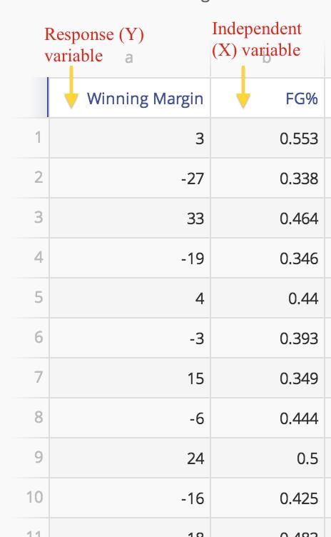
• Y = the dependent (response/ (output) variable
• a = the y-intercept (a constant or baseline, giving the value of Y when X = 0)
• b = the regression coefficient (slope) representing the amount of change in Y for a 1-unit increase in X
• X = the independent (explanatory/predictor/input) variable
• e = error term representing the unexplained or residual variance.

The parameters ‘a’ and ‘b’ are calculated using the Least Squares method, a mathematical routine that plots a line of best fit to the data by minimizing the variability of the data about that line.

Using EngineRoom

Note: The example below is worked out with the Guided Mode disabled, so it combines some steps in one dialog box. You can enable or disable Guided Mode from the User menu at the top right of the EngineRoom workspace.

To use the tool, select the Analyze menu > Regression Analysis... > Simple Regression. The study opens on the workspace:

There are two 'drop zones' attached to the study:

• Response Variable (required): for the variable containing the output measurements. Must be numeric (and is assumed continuous).
• Independent Variable (required): for the variable containing the input levels or measurements. Can be numeric or text.

Example:

The example dataset contains data collected over 22 days on an output variable (Y), Customer Satisfaction Rating, and an input variable (X), Days to Pay Claim, along with the observation numbers (Data Pair). We will analyze these data to see whether Days to Pay Claim (X) accounts for the bulk of the variation in Customer Satisfaction (Y).

Steps:

• Open the Simple Regression tool onto the workspace.
• Click on the data file in the data sources panel and drag ** Days to Pay Claim** onto the Independent Variable drop zone.
• Drag Customer Satisfaction Rating onto the Response Variable drop zone.
• Enter the value of the desired risk or significance level (this should be a value between 0 and 1, conventionally 0.05 or 0.1) or leave the default value of 0.05 as is.
• Click Continue

Note: Nominal variables (categorical with multiple levels) must be converted to binary indicator/dummy variables before using them in the analysis.

The Simple Regression Analysis includes graphical and numeric output:

The model is significant (p-value = 0) and explains over 60% of the variation in Customer satisfaction (R-squared = 0.61)

The graphical output contains:

• Scatter plot of the input (X = Days to Pay Claim) vs. output (Y = Customer Satisfaction Rating) showing the line of best fit.

And three residual plots:

• Normal Q-Q (quantile- quantile) plot which is like a probability plot. If the plotted points fall along the diagonal line, the assumption that residuals are normally distributed, holds.
• Scatter plot of Standardized residuals vs. the time order of the observations. If the plotted points are randomly scattered with no patterns or trends, the assumption of independent residuals holds.
• Scatter plot of Standardized residuals vs. fitted values (predictions of the data observations using the regression model). If the plotted points are randomly scattered with no patterns or trends, the assumption of independent residuals holds.

The numeric output contains:

• Regression model expressed as a line equation
• Regression statistics table showing the correlation coefficient (r ), coefficient of determination (R-square = R^2), Adjusted R-square (adjusted for the total number of X variables in the model) and the count (sample size)
• Coefficient Table
• ANOVA Table

Instructor Resources

PowerPoint Download