Non-normal Process Capability Analysis - Continuous Data Tutorial

Tutorial

Coming Soon

Click to Download Data File

When to use this tool

Use the Non-normal Process Capability Analysis - Continuous tool to assess the capability of a continuous process to meet customer requirements or specifications when the process data have a non-normal distribution. The output from this study includes an overview of process stability, the best-fit non-normal distribution, and the process capability.

How to use this tool in EngineRoom

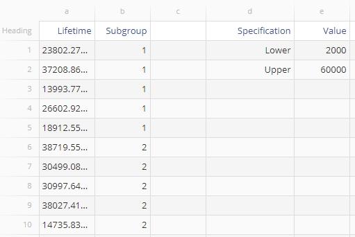
We will use the example data set provided above to run the capability analysis. Upload the example data provided into EngineRoom. The data set has two columns - ‘Lifetime’ contains the observed lifetimes in hours of 200 motors, and ‘Subgroup’ contains the corresponding subgroup labels. We will first run the analysis using subgroup size of 1 (individual observations) followed by subgroup sizes of 5.

Example using Individuals Data:

1. Open the Non-normal Process Capability Analysis - Continuous tool, located in the Measure (DMAIC setup) menu or Quality Tools (Standard) menu, in the Process Capability submenu:

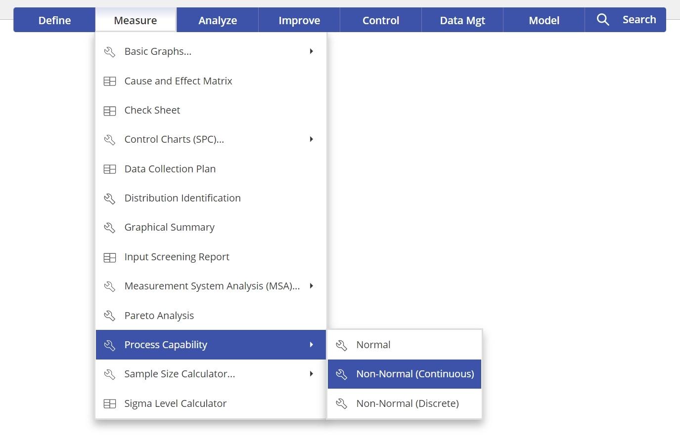
2. Click on the Non-Normal Process Capability tool to open it in the workspace.

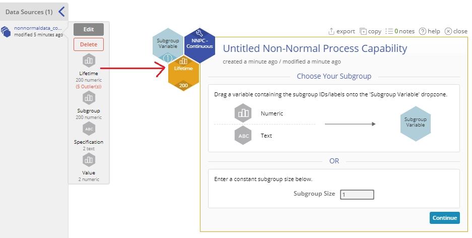
3. From the data sources Variable panel, drag the numeric ‘Lifetime’ variable on to the Data Variable hexagon dropzone.

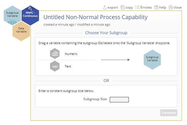
4. Now you can drag a numeric or text subgroup ID variable identifying the subgroups on to the Subgroup Variable drop zone OR Enter a constant subgroup size in the data entry box provided for this value. If you do not have subgroups, enter ‘1’ into this box.

For this example, enter the value ‘1’ in the Subgroup Size text box and click Continue.

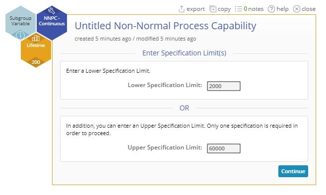
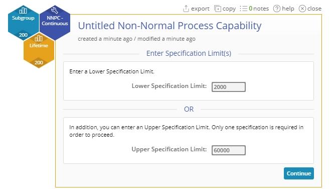
5. On the 'Enter Specification Limit/s' screen, enter the value for AT LEAST ONE specification (lower and/or upper) limit in the designated text boxes. For the example data, enter the specification limits as ‘2000’ and ‘60000’ as shown and click Continue.

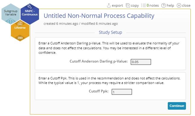
6. On the 'Study Setup' screen, you have the option to change the default values of the cut-offs for deciding the Anderson Darling Goodness-of-fit Test and the minimum acceptable Ppk capability statistic. For the example, leave the default values in and click Continue.

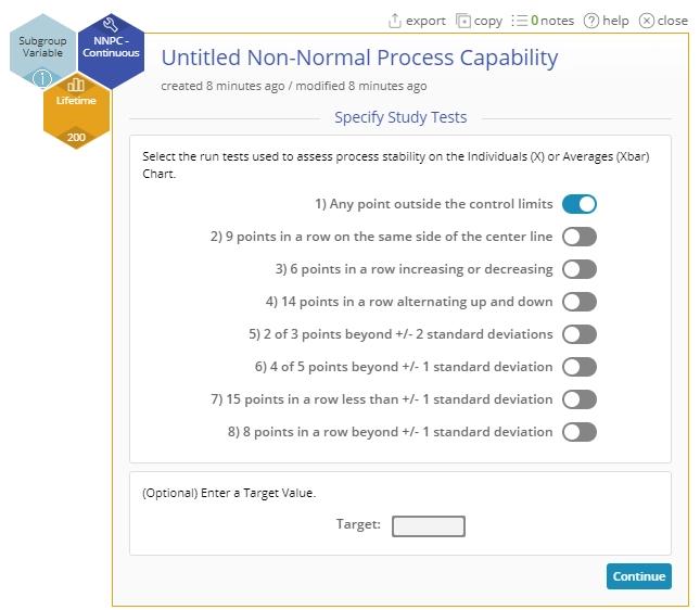
7. On the ‘Specify Study Tests’ screen, select the desired tests for checking the stability of the process - only the first test ('Any point outside the control limits') is chosen by default. In addition, you can enter an optional Target value for the process on this screen.

8. Click the Continue button in the dialog. The first part of the output for the identifies the best-fit and second-best fit non-normal distributions:

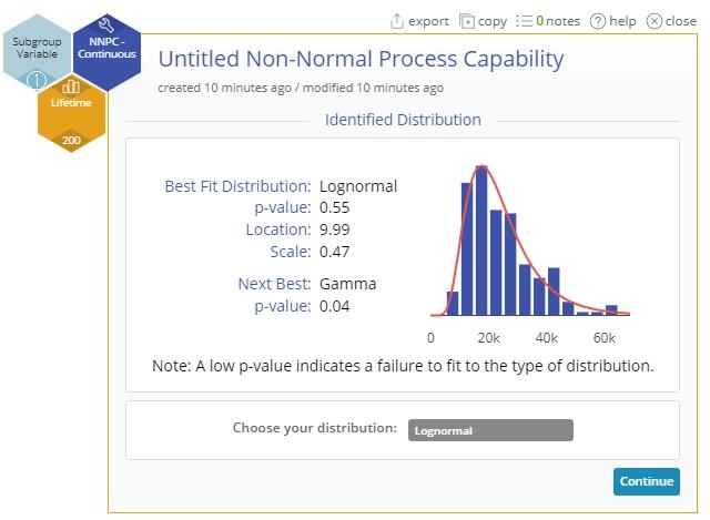
9. To continue with the identified distribution, simply click Continue. You can also change the fitted distribution using the drop-down menu provided. Click Continue. The Non Normal Process Capability Analysis output is shown:

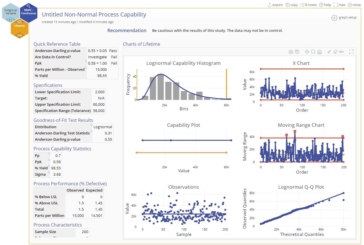
The Output

The output includes:

1. A recommendation statement at the top highlighting any issues.

2. Quick Reference Table showing the key results:

• The goodness-of-fit p-value compared with the specified cut-off, along with the recommendation (Pass or Fail)
• A determination of whether the data pass the control chart tests with a recommendation to investigate the causes if the data fail any tests.
• The performance or capability statistic Cpk or Ppk and a result of Pass or Fail based on the prespecified cut-off value.
• The observed Parts Per Million (PPM) or defective product calculated from the data.
• The Percent Yield or amount of the process falling between the specification limits.

3. Specifications: shows the entered specification limits and their range (tolerance).

4. Goodness-of-Fit Test Results: shows the best-fit distribution (or the chosen distribution if you changed it) along with the goodness-of-fit test statistic and corresponding p-value.

5. Process Capability Statistics: shows the Pp, Ppk, % Yield and Sigma Level values.

6. Process Performance (% Defective): shows the percentage of the process below the lower specification limit (LSL) and above the upper specification limit (USL) for the observed and expected (fitted) distribution. The total % defective is also computed and then converted to parts per million (PPM).

7. Process Characteristics: shows the sample size, subgroup size, number of subgroups, sample mean and standard deviation from the data.

8. Distribution Parameters: shows the fitted distribution name along with its defining parameters (location, shape and scale as appropriate.)

The graphs in the output are as follows (descriptions of the three graphs in the left column followed by those in the right column):

• A histogram of the data overlaid with the fitted distribution curve. The specifications are shown as reference lines.
• A capability plot comparing the process spread (blue line) with the specification range or tolerance (orange line).
• A run chart showing the individual observations or subgroup averages over time to assess the independence of the observations.
• Control charts based on the subgrouping structure of the data: X and mR charts for individuals data and Xbar and R or S charts for subgrouped data.
• A Quantile-Quantile (Q-Q) Plot assessing the fit of the data to the chosen non-normal distribution.

Example using Subgrouped Data:

Now let’s run the same analysis by considering the subgroups in the dataset under the Subgroup column. Re-run the analysis using the steps for the individuals data, but this time drag the Subgroup variable onto the Subgroup Variable hexagon on the study:

Notes:

• A subgroup contains the items measured together at the same time, under the same conditions. The subgroup variable identifies these subgroups in your data; for example, if you measure five parts coming off the production line every hour, your subgroup variable labels the first five parts as '1', the next five parts as '2', etc.
• Instead of dragging on a subgroup variable, you can enter the appropriate numeric value in the Subgroup Size box: if you measure five parts coming off the production line every hour, your subgroup size is 5. If you only measure one item per time period, your subgroup size is 1.

Important: Your subgroups must all be the same size for this analysis to run.

The remaining steps and inputs are the same as before. The output for the subgrouped data is shown:

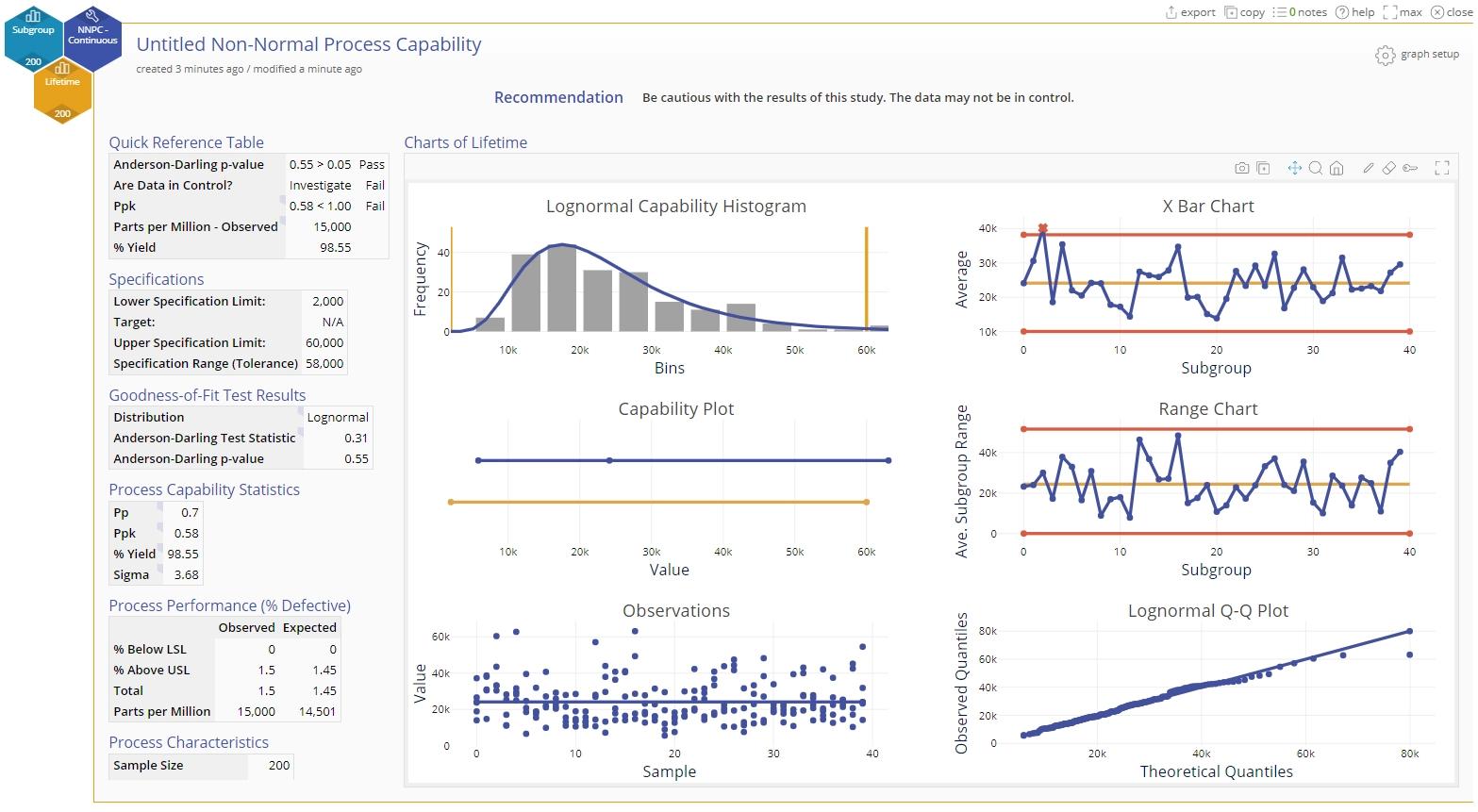
Note: The best-fit distribution, capability/performance statistics and % Defective or % Yield values stay the same as before in the individuals data case. The only change is in the control charts displayed (Xbar and R or S charts are used for subgrouped data) and the averages are now plotted on the Observations chart. Interpretation of these charts is similar to before - any out of control points on the control charts indicate an unstable process and trends or patterns on the Observations chart indicate non-randomness or non-independence in the data.