
Example: Full Factorial DOE
When to use this tool
Use the full factorial DOE to analyze the effects of multiple factors, each at two levels, on a numerical response. These designs are best used when you have few factors (up to 4 or 5), since they can get quite large and cost prohibitive.
The advantage of full factorial designs is that they can estimate all main effects and interaction effects without aliasing (confounding with other effects).
An Example Using EngineRoom
Example:
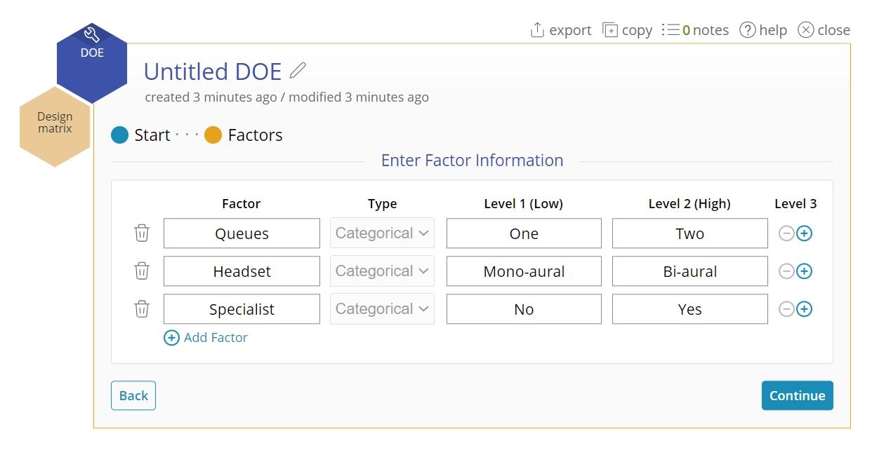
In this example, we will create and analyze a full factorial to reduce wait times. There are three factors being studied at two levels each:
- Number of Queues: One/Two
- Type of Headset: Mono-aural/Bi-aural
- Extra Specialist: No/Yes
Steps:
1. Create Design:
- Open the DOE tool
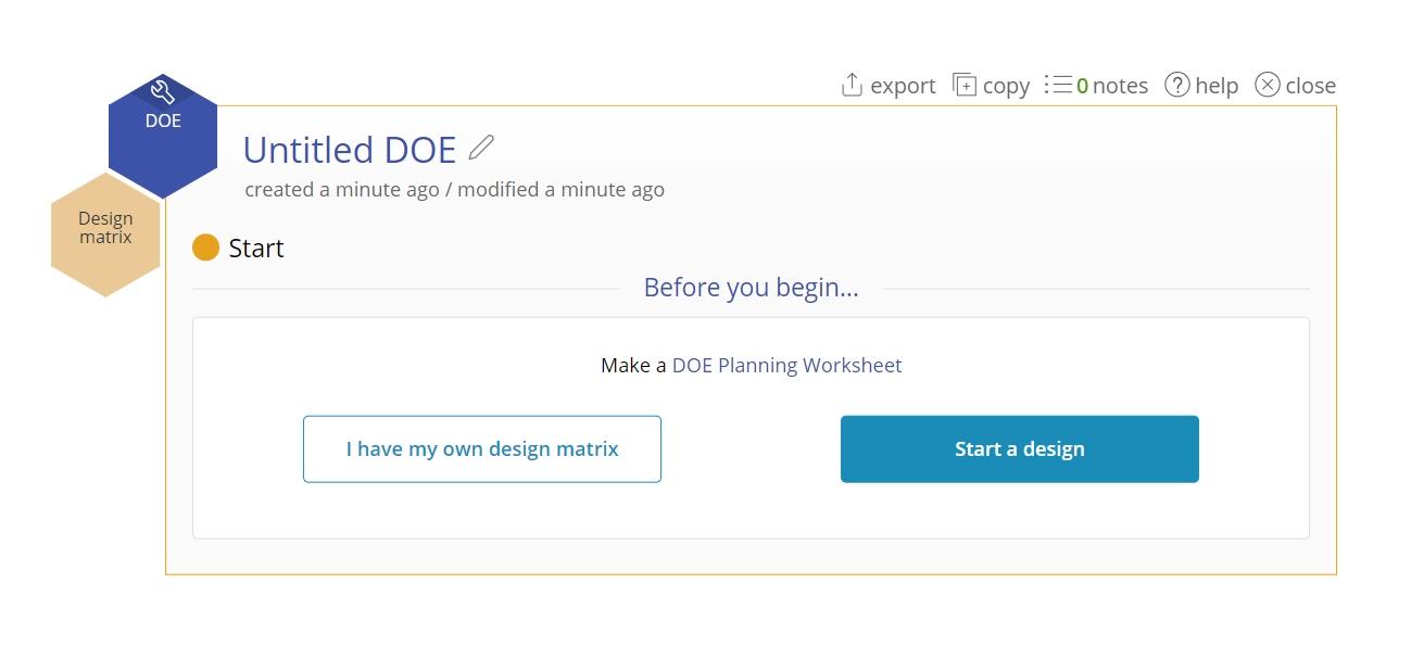
- Select Start a design
- Add your factors from the study
- Select the Full design corresponding to 3 factors, which gives 8 runs:
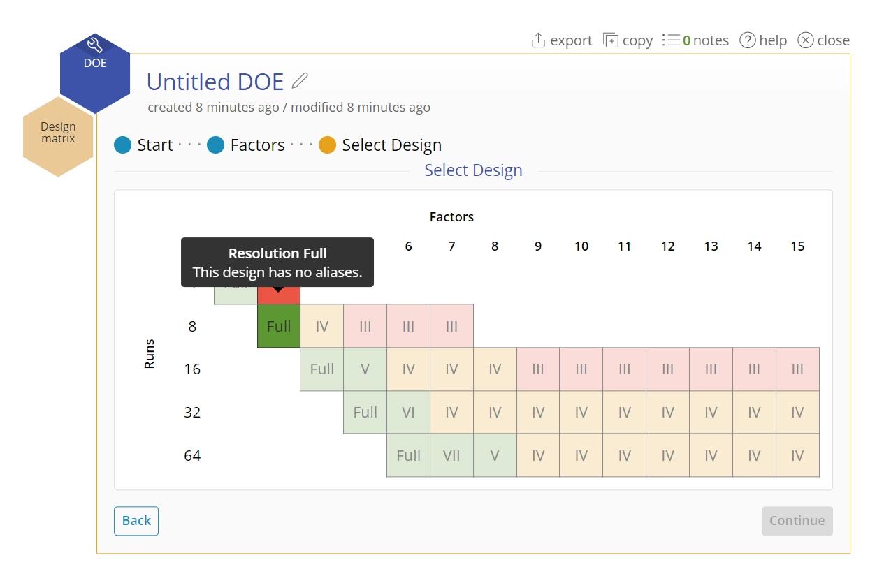
- Complete the settings for the design as shown below. The design will be run at two different locations (centers) so we will create two replicates of the design. Also, selecting 2 blocks will account for the variability from the replicates.

- Notice how you have over 90% power to detect an effect size of 2 standard deviations.

- Click Create Design.
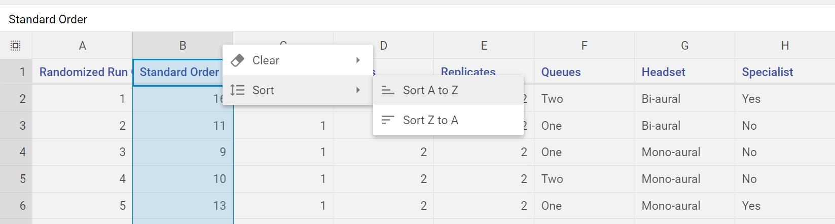
2. Enter Data:
- The design matrix opens up from the data sources panel. It contains all the information about the design, with a blank column at the end; normally you would run the experiment by following the Randomized run order, and enter the response data into this column. However, since we already have the response data, we want to organize the table into Standard Order. This way we can simply enter or copy-paste the data, since the run order of both designs is identical (i.e., run #1 in the design we just created is the same as run #1 in the design table provided.) Sort the created design in the Standard order as well by right-clicking on the Standard order column, and clicking Sort > A -> Z:
- Copy-paste the response data into the blank column and click the "save and close" button:

3. Analyze Design:
Now it's time to analyze the design.
Note: If you need to change the design, you can click on the navigation across the top, or the Back button.
- Drag the Design matrix variable from the data sources panel onto the Design matrix drop zone, and the Wait Time variable onto the Response Variable drop zone. Click Continue.
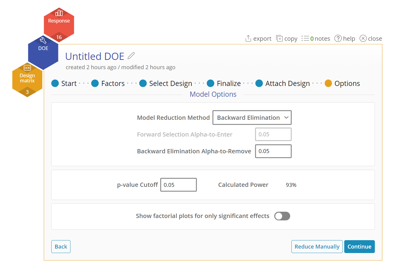
- Adjust any of the following parameters:
- Model Reduction Method: The default is to use Backward Elimination to reduce the model from full to the most significant factors. Other options include Forward Addition, Stepwise, and Manual Reduction.
- p-value: This option allows you to change the p-value after the creation of your design. You can see the new power calculated next to it.
- Show only Factors in Model: This has plots that only show within the model.
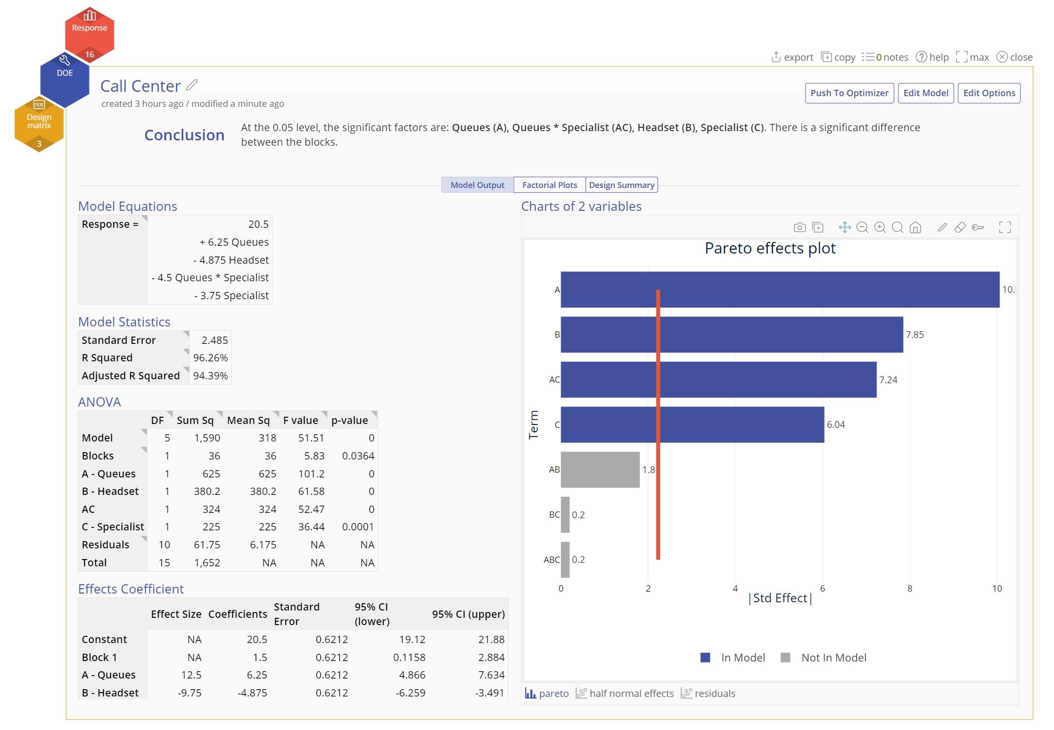
- The output contains several parts.
- Model Output Screen: This screen shows the resulting model equations and various factors the indicate the significance of an input.
Pareto effect plot:
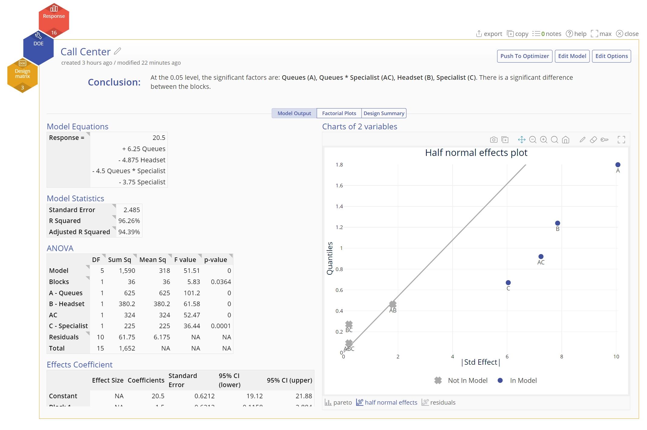
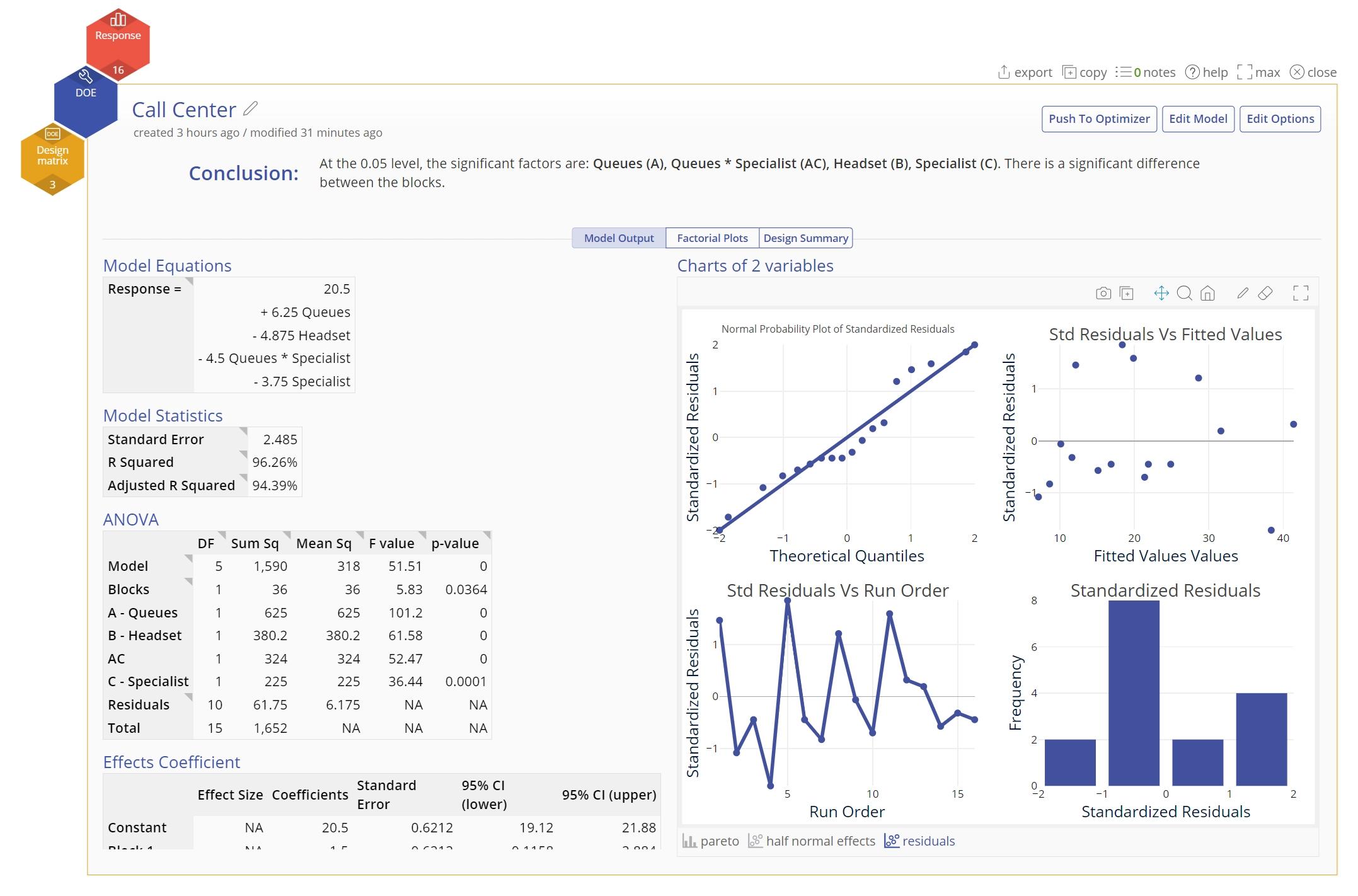
There are additional graphs that can be found on the tabs at the bottom.
Half normal effect plot:
Residuals plot:
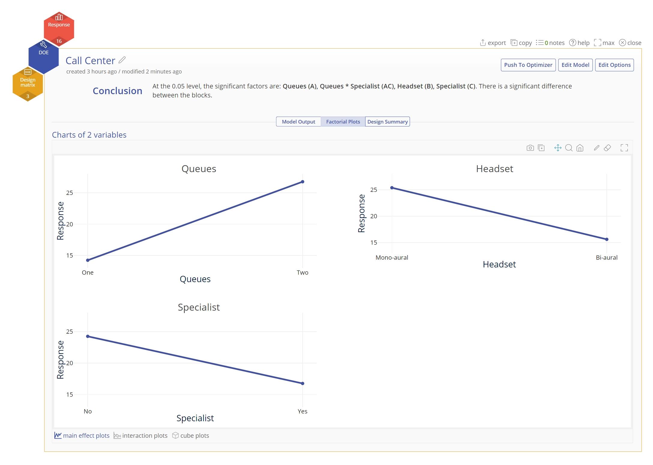
- Click on the Factorial Plots tab to see the main effect and interaction plots:
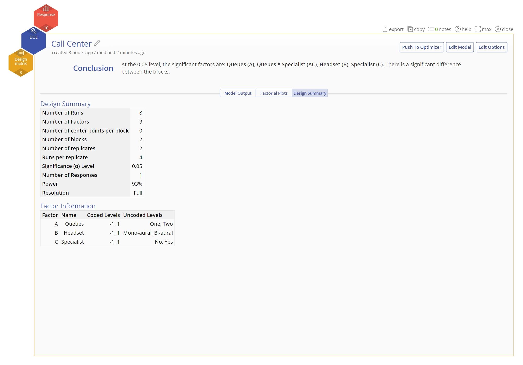
- Click on the Summary tab to see the design summary:
- Select the Edit Model or Edit Options button at the top right of the study to edit the model further or to change any of your previously selected model selection settings:
Push to Optimizer
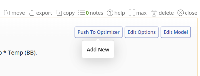
From here you can use the Push to Optimizer button to optimize the output.
1. Click on the Push to Optimizer button on the top right.
Learn more about the Response Optimizer.
Tutorial
Full Factorial DOE Tutorial
Was this helpful?