Multiple Regression Analysis Tutorial

Tutorial

Click to Download Data File

When to use this tool

Use Multiple Regression Analysis to explain the relationship between one continuous dependent/output (Y) variable and multiple independent/input (X) variables. The responseoutput variable is assumed to be continuous.

Multiple Regression analysis models the data using a linear equation of the form

where

• Y = the dependent output or response variable; assumed to be continuous
• a = the constant term (value of Y when all inputs are set to zero)
• X1, X2, .…Xk = the k independent inputs or predictor variables. These can be continuous or categorical.
• b1, b2, ...bk = the coefficients corresponding to the k inputs
• e = error or unexplained variance

Using EngineRoom

Note: The example below is worked out with the Guided Mode disabled, so it combines some steps in one dialog box. You can enable or disable Guided Mode from the User menu at the top right of the EngineRoom workspace.

To use the tool, select the Analyze menu > Regression Analysis... > Multiple Regression. The study opens on the workspace:

There are two 'drop zones' attached to the study:

• Response Variable (required): for the variable containing the output measurements. Must be numeric (and is assumed continuous).
• Independent Variables (required): for the input or independent variables used to explain or predict the output. You must have at least two independent variables on this drop zone, or the analysis will not run. All Xs must be numeric; binary variables must be coded 0/1.

Note:

1. Nominal (categorical with multiple levels) X variables must be converted to binary indicator/dummy variables before using them in the analysis.

Example:

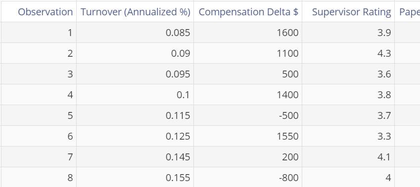
The example dataset contains data on the annual turnover rate among nurses, along with observed data on several potential ‘explanatory’ variables such as Compensation, Supervisor Rating, Paperwork Burden (%), etc. We will analyze these data to see whether the X variables account for the bulk of the variation in nurse turnover.

Steps:

• Open the Multiple Regression tool onto the workspace.
• Click on the data file in the Nurse turnover data source and drag each of the input variables, Compensation Delta, Supervisor Rating, Paperwork Burden, Working Hours Per Week and Patient/Nurse Ratio onto the Independent Variables drop zone.
• Drag Turnover (Annualized %) onto the Response Variable drop zone.
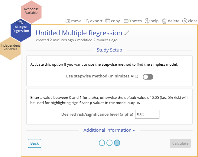
• At this point you can select the Best Subsets method to automate the model selection and arrive at the best model based on the best subsets method. Do not select this option yet.
• Enter the value of the desired risk or significance level (this should be a value between 0 and 1, conventionally 0.05 or 0.1) or leave the default value of 0.05 as is. Let’s use the default value in this case.
• Click Continue

Output:

All of the X variables dragged on to the study are included in the model. The significant p-values are flagged as shown:

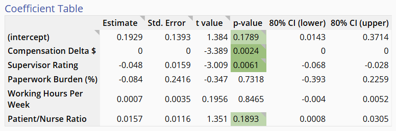
At this point you can simplify the model manually by dragging off individual non-significant X variables one at a time until all the terms remaining in the model are significant.

Alternatively, you can click the Study Setup button within the top right corner of the study to open the panel and select the option ‘Use best subsets method’ to select the model for you. Doing so and clicking ‘Save changes’ displays the final model with only the significant terms included:

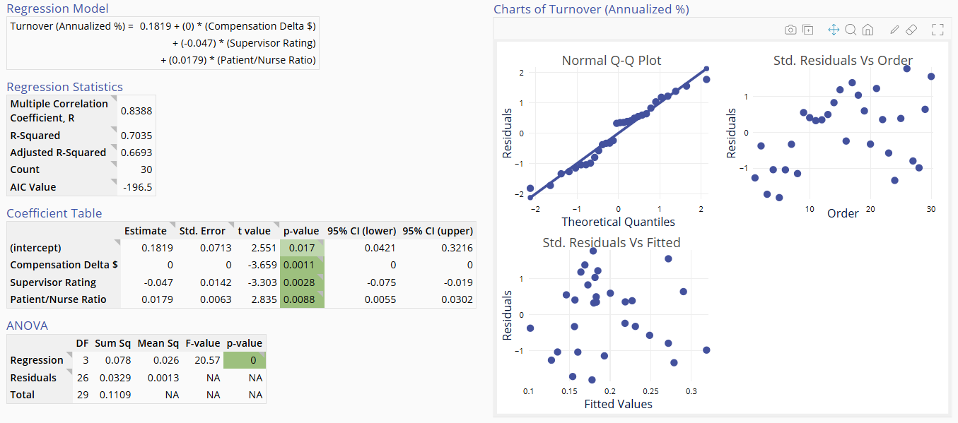
The Multiple Regression Analysis output includes graphical and numeric output.

The graphical output contains three residual plots:

• Normal Q-Q (quantile- quantile) plot which is like a probability plot. If the plotted points fall along the diagonal line, the assumption of normally distributed residuals holds.
• Scatter plot of Standardized residuals vs. the time order of the observations. If the plotted points are randomly scattered with no patterns or trends, the assumption of independent residuals holds.
• Scatter plot of Standardized residuals vs. fitted values (predictions of the data observations using the regression model). If the plotted points are randomly scattered with no patterns or trends, the assumption of equal variances holds. This plot is also used to detect non-linearity and outliers.

The numeric output contains:

• Regression model expressed as a mathematical equation
• Regression statistics table
• Coefficient Table
• ANOVA Table
• Variation Inflation Factor table
• Variables Not in Model table (shown only if the automated best subsets option is chosen)

Instructor Resources

PowerPoint Download