Non-normal Process Capability Analysis - Discrete Tutorial

Tutorial

Coming Soon

Click to Download Data File

When to use this tool

Use the Non-normal Process Capability Analysis - Discrete tool to assess the capability of a process to meet customer requirements or specifications when the process data have a discrete distribution, such as Binomial or Poisson. These distributions are based on counts of things.

The Binomial distribution describes the counts of defective items (or events) when each item can either be defective or not. The total number of defectives in this case cannot exceed the total number of items. The Poisson distribution describes the counts of defects per item, when each item can have more than one defect. The total number of defects in this case can exceed the total number of items.

The output from this study includes an overview of process stability, the Percent Defective or Defects per Unit trends over time, and the process capability.

How to use this tool in EngineRoom

We will use the example data provided above to run the Discrete data capability analysis. Upload the example data provided into EngineRoom.

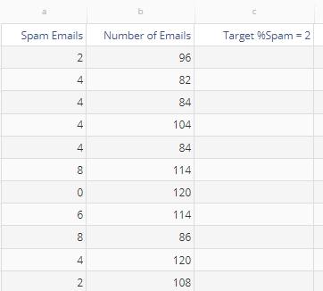
Binomial (Defectives) Data

The Binomial data set contains the number of spam emails and the total number of emails received in an account per day. We will first run the analysis using the variable sample sizes (number of emails) provided, and then run it again using a constant sample size of 100.

Example using Binomial (Defectives) Data and Unequal Sample Sizes:

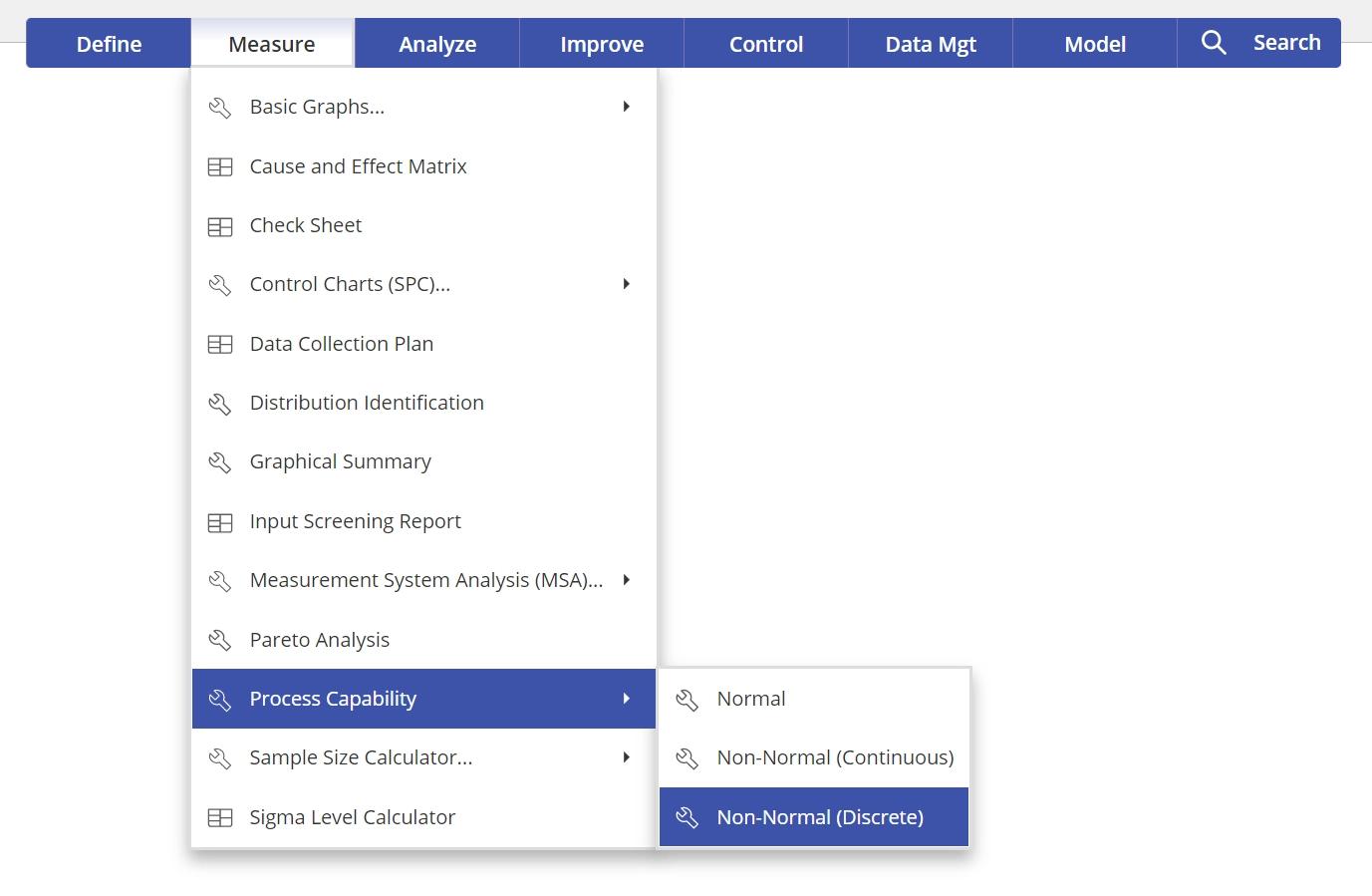
1. Open the Non-normal Process Capability Analysis - Discrete tool, located in the Measure (DMAIC setup) menu or Quality Tools (Standard) menu, in the Process Capability submenu:

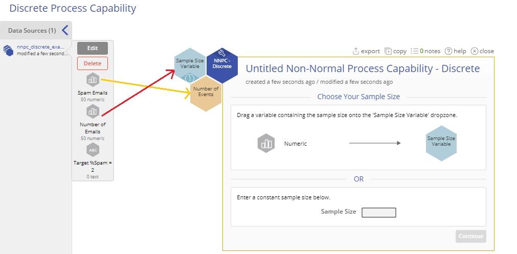
2. From the data sources variable panel, drag the Spam Emails variable on to the Data Variable hexagon dropzone.

3. Next, drag a numeric sample size variable onto the Sample Size Variable hexagonal drop zone OR Enter a constant sample size in the data entry box provided for this value. For this example, drag the ‘Number of Emails’ variable onto the Sample Size Variable hexagonal drop zone and click Continue.

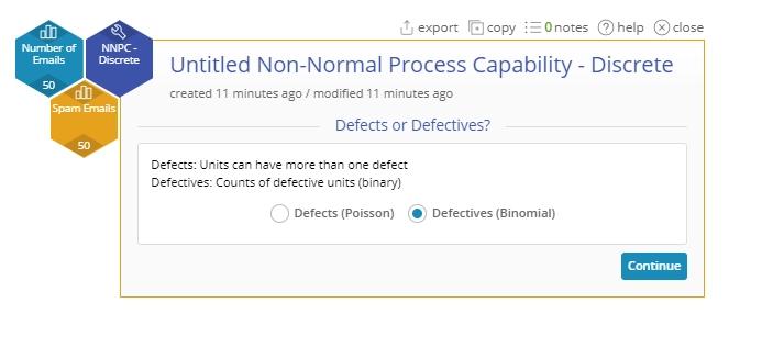
4. Select the appropriate option based on whether you’re counting defects or defectives - in this case an email is either spam or it isn’t, so select Defectives:

5. On the ‘Specify Study Tests’ screen, select the desired tests for checking the stability of the process - only the first test ('Any point outside the control limits') is chosen by default. In addition, you can enter an optional Target value for the process on this screen. For our example, enter the target %Spam value as 2, i.e., we want to target 2% spam or lower.

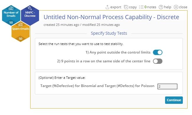
6. Click Continue to see the output:

Output

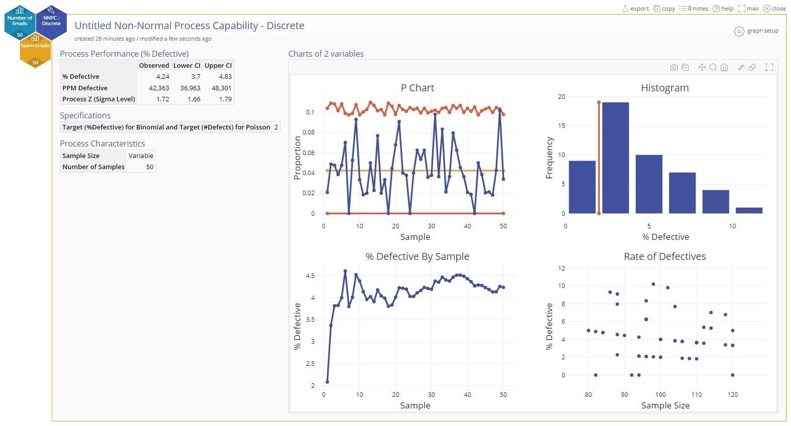
The output includes numeric tables and four graphs:

The output graphs are as follows (left to right starting from top row):

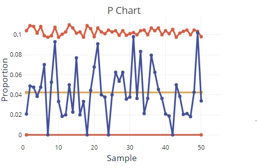
• A p-chart of the proportion defective data with a center line at the mean (average) proportion defective and upper and lower control limits based on the samples. In this example, our sample sizes are variable, so the control limits appear jagged to reflect the varying sample sizes.

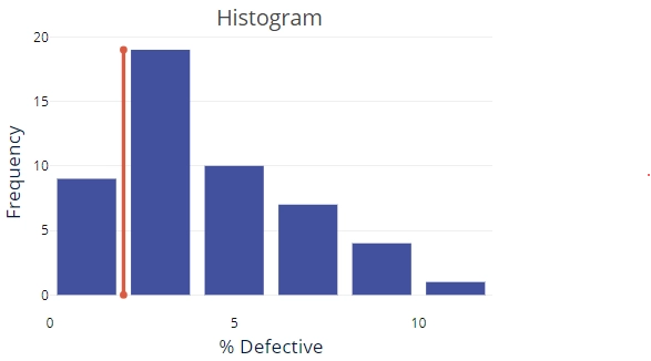
• A histogram of the %Defective (in our case, %Spam) data with the target (if provided) shown as a reference line.

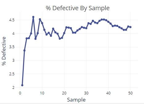
• A graph of the %Defective for each sample, in the order that the samples were collected. Use this graph to determine whether you have enough samples for a stable estimate of the %defective. If the %defective line flattens out over the course of time as you collect more samples, then the %defective is stable.

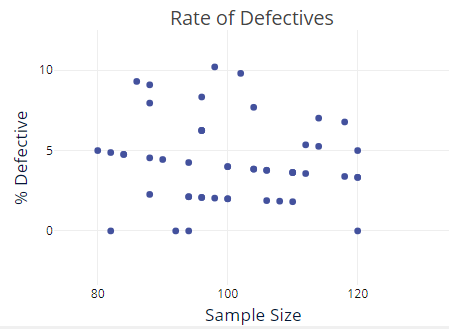
• If the sample sizes vary as in this case, the last graph plots the %Defectives against the sample size. Use this graph to check the assumption of a Binomial distribution that the probability of a defective item is constant across different sample sizes. If the %Defective data are randomly distributed across sample sizes without any trends or patterns and randomly scattered about the horizontal center line, the data follow a Binomial distribution.

Example using Binomial (Defectives) Data and a Constant Sample Size:

Open the Non-normal Process Capability Analysis - Discrete tool and from the data sources variable panel, drag the Spam Emails variable on to the Data Variable hexagon dropzone. Next, enter the constant sample size of ‘100’ in the Sample Size box and click Continue. Repeat the remaining steps as above to get the output:

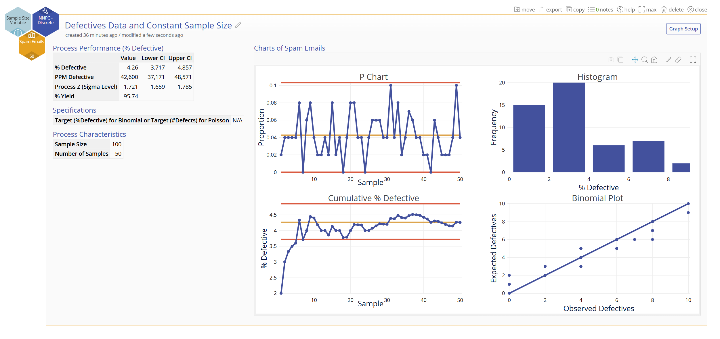
The output is essentially the same except for two items:

• The p-chart now has a solid line representing the upper control limit, reflecting the fact that the sample size is the same for all samples.
• Instead of a ‘Rate of Defectives’ graph, we now have a Binomial Plot showing the number of observed defectives (spam emails in our example) per sample compared against the expected number of defectives per sample from a Binomial distribution. Use this graph to check whether your data follow a Binomial distribution. If the plotted points fall along the diagonal line, the data follow a Binomial distribution.

Poisson (Defects) Data

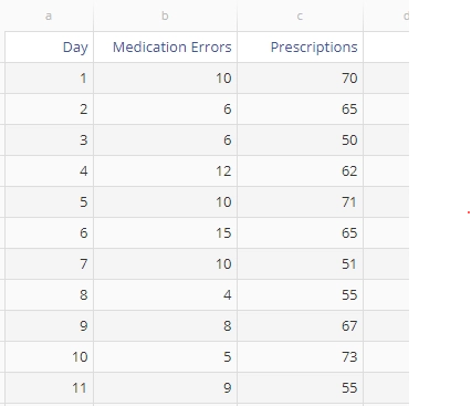
The Poisson data set contains the number of medication errors and the total number of prescriptions ordered per day for 50 days. We will first run the analysis using the variable sample sizes (number of prescriptions) provided, and then run it again using a constant sample size (number of prescriptions per day) of 60.

Example using Poisson (Defects) Data and Unequal Sample Sizes:

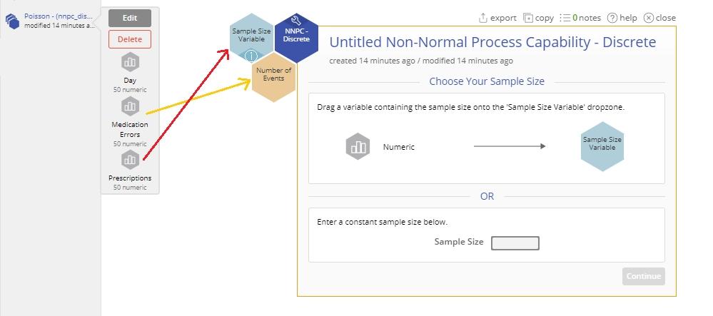
1. Open the Non-normal Process Capability Analysis - Discrete tool.

2. Drag on the Medication Errors variable onto the Data Variable drop zone and the Prescriptions variable onto the Sample Size Variable drop zone.

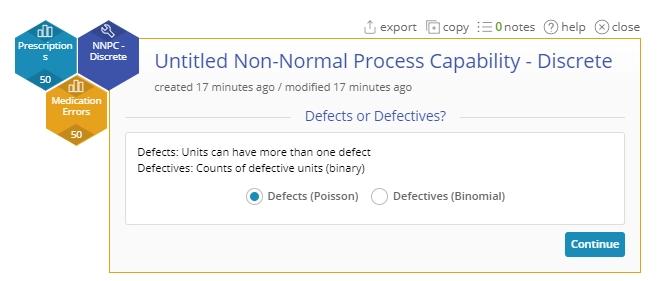
3. Select Defects on the next screen to specify a Poisson distribution for the errors data.

4. On the ‘Specify Study Tests’ screen, enter the Target value for the process as 0, i.e., we want to target 0 medication errors per prescription ordered.

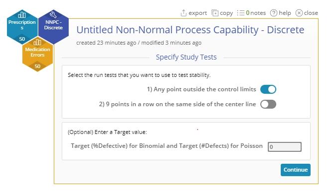
5. Click Continue. The output is shown:

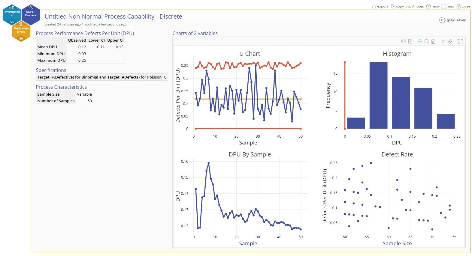
Output

The output contains the following:

The output graphs are as similar to the corresponding Binomial case:

• A u-chart of the Defects per Unit (DPU) with a center line at the mean (average) DPU and upper and lower control limits based on the varying sample sizes.
• The remaining graphs are interpreted just as in the Binomial case , but now applied to Defects per unit (DPU).

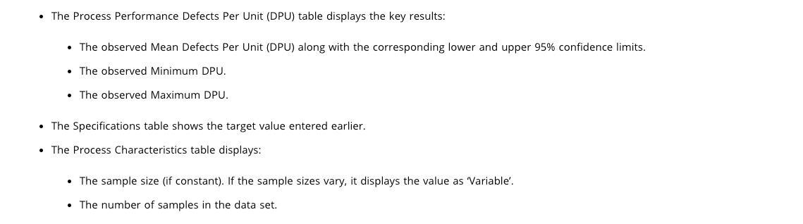
Example using Poisson (Defects) Data and a Constant Sample Size:

For this example, repeat the steps from the previous section, except instead of using the Prescriptions variable, enter the value ‘60’ in the Sample Size box and click Continue to get the output:

Once again, the output shows shows minor changes reflecting the constant sample size:

• The u-chart has a constant upper control limit (solid line).
• Instead of a ‘ Defect Rate’ graph, we now have a Poisson Plot showing the number of observed defects (medication errors in our example) per sample compared against the expected number of defects per sample from a Poisson distribution. Use this graph to check whether your data follow a Poisson distribution. If the plotted points fall along the diagonal line, the data follow a Poisson distribution.

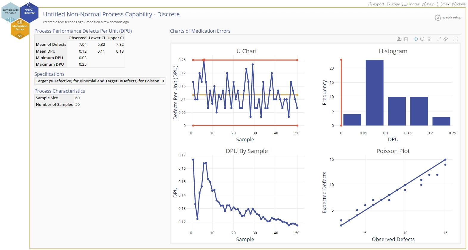
Note: Once a study is created, you can always change the settings for the analysis by clicking on the 'graph setup' button at the top right of the study window: