Impact of Variation, Labeling

Impact of Variation, Labeling: A simple model for instructional purposes to demonstrate the impact of variation in time by comparing two different stems of a process. Two lines of a labeling process have the same mean processing time but different amounts of variation in the time to process.

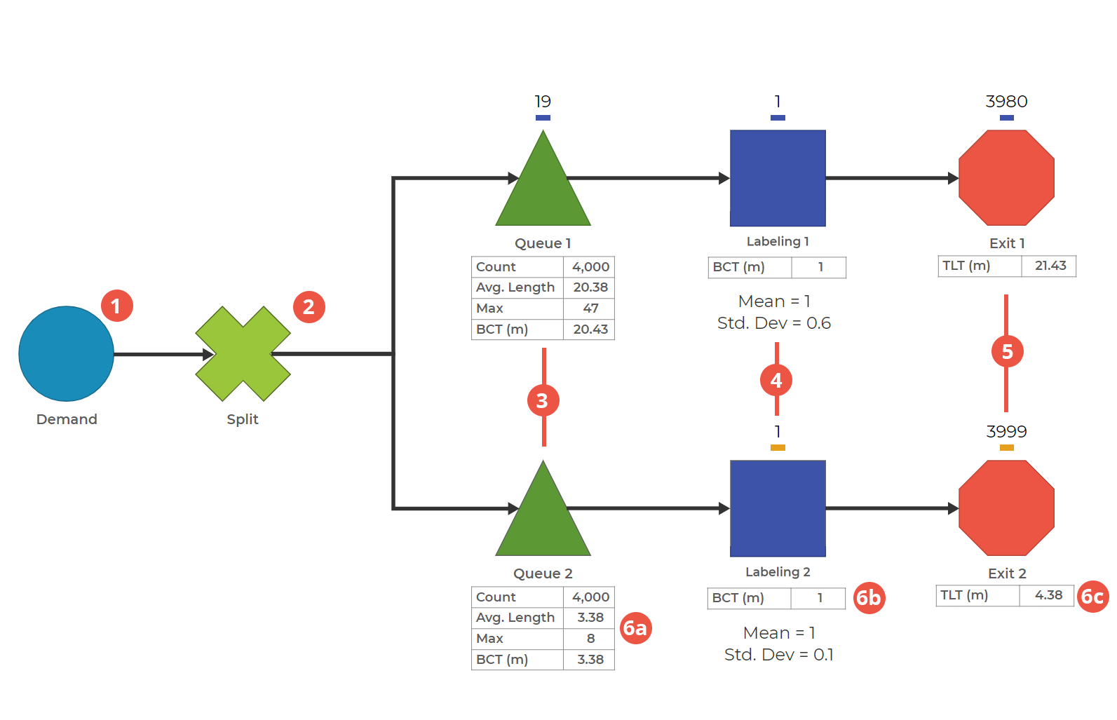
0. There are three items in this process. Combined Item, Line 1 Item, and Line 2 Item. The Combined Item consists of one Line 1 Item and one Line 2 Item. The goal of this configuration is to ensure both lines have the exact same demand.

1. Set the rate of the Combined Item. This Demand Block creates one Combined Item every minute, with a constant distribution.

2. Split the Combined Item to feed both lines with the same demand. Using both the Combined Item and Split Block guarantees that both lines get the same demand rate. This step is especially useful if we change the Demand from a constant distribution to one with variation.

3. Set the Queues to accept only one type of item. Queue 1 only accepts Line 1 Item, and Queue 2 only accepts Line 2 Item. 

4. Model the variation in the Labeling Activities. Both Activity blocks label items with a mean time of 1. However, Labeling 1 has a Standard Deviation of 0.6, and Labeling 2 has a Standard Deviation of 0.1. While both are using Normal Distributions, Labeling 2 is running with less variation than Labeling 1.

5. End the process. Add Exit Blocks to capture the final results of the process.

6. Run the process and check out the statistics. This model will run for 4000 minutes.

6a. Queue Block Statistics:

• The Count of both Queue Blocks is equal. This means both Queue Blocks had the same number of items pass through.
• Queue 2 has a lower Average Length than Queue 1. Average Length refers to the average number of items in the Queue Block throughout the simulation.
• Queue 2 has a lower Max than Queue 1. Max refers to the maximum number of items in the Queue Block at any point in the simulation.
• Queue 2 has a lower average Block Cycle Time (BCT) than Queue 1. BCT refers to the amount of time an item spends in a block. This table shows the average BCT for all items that pass through that block.

6b. Activity Block Statistics: 

• The Block Cycle Time (BCT) in both Activity Blocks is equal. BCT refers to the amount of time an item spends in a block. This shows that an item was in the labeling process for 1 minute, on average, regardless of which line the item was on. If you'd like to see the variation in the BCT, check out the Block Cycle Time graph in the Results (not shown).

6c. Exit Block Statistics:

• Exit 2 has a lower average Total Lead Time (TLT) than Exit 1. TLT refers to the time an item spends in the process before arriving at the block. For example, a TLT of 4.38 at Exit 2 means that, on average, the items spent 4.38 minutes in the process before arriving at Exit 2.

The only difference between the two lines is the amount of variation in the labeling step. Process planning often uses averages, but it's not usually the average (mean) that causes problems; it's the variation around the average. A simulation like this can show how other metrics in the process, like WIP and Lead Time, are affected by increased variation and how much better the flow is with reduced variation.

Note: If you build this model, your numbers will be different due to the variability.