How to Conduct an MSA When the Part is Destroyed During Measurement

Introduction

Gauge R&R is a well-known procedure for evaluating measurement systems. It breaks down the total process variation into its components:

• part‐to‐part or process variation
• appraiser variation (reproducibility)
• measurement system variation (repeatability) and
• under the ANOVA method, the appraiser‐by‐part variation

The general and most commonly used form of the study, called a Crossed Gauge study, consists of repeated measuring of the same parts by multiple appraisers. This form of study assumes that the parts are preserved in their original condition and do not undergo any changes, physical or otherwise, between trials or between handoffs (between appraisers)

Under most situations, this is a relatively safe assumption to make, but what happens when measurement of the same parts cannot be replicated for some reason, such as when the part is destroyed or incontrovertibly changed when it is measured? For example, to test the strength of a weld, you must bend it until it breaks or stretch polymer fibers until they tear to measure tear resistance. A crossed study is impossible in these situations as no part can be measured twice. So, how do you conduct a measurement system analysis when the part is destroyed during measurement?

The form of gauge study used in destructive scenarios is called a Nested Gauge R&R study, wherein each appraiser measures a different sample of parts but where the parts of each type are assumed to be very similar (homogenous).

An Example of Nested Gauge R&R

A manufacturer of prosthetic devices has commissioned a study to evaluate the measurement system used to test the hardness of the reinforced plastic parts on the devices. The test involves subjecting a sample of randomly selected parts to a pre-specified force on a standardized presser foot. A durometer is used to measure the depth of the indentation in the material created by the force, and the score is recorded (the score is a unitless number on a scale of 0‐100, with higher scores indicating greater hardness). The operating range for the process is 30‐45.

The parts for the devices arrive in lots of 50. Since the sampled parts are destroyed as part of this process, a nested sample is appropriate. Three appraisers are randomly selected to do the measuring. Five lots are picked to represent the full range of the process. Six parts are selected from each lot, two for each appraiser. The design is as shown below:

Note that although each appraiser measures parts from the same five lots, the actual parts measured from each lot are different. For instance, of the six parts selected from lot 1, two parts at random are assigned to appraiser A, two parts to appraiser B and two parts to appraiser C. The six parts from lot 2 are similarly assigned to the three appraisers. The measurements made by each appraiser on the parts from each lot are treated as repeated measurements or trials on the 'same' part.

Obviously, these are not true repeated measurements, but because the parts came from the same lot in close proximity to each other, they're assumed to be nearly identical i.e., they represent the same part for all practical purposes. Thus the parts within a lot are very similar and the parts from different lots are as dissimilar as possible.

A Nested Anova is the appropriate procedure for the analysis of a destructive study, because it recognizes that the samples are nested within the appraisers — each appraiser tests a different sample from the same lot. The Nested Anova procedure is easily available in most statistical software programs. The following results were obtained using Minitab®'s "Gauge R&R (nested)" procedure.

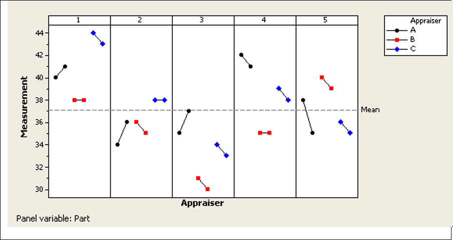
Let us examine the Gauge Run chart — this chart allows you to see the individual measurements made on each part by the individual appraisers. For purposes of this graph, the six parts from each lot were labeled with the lot number (so the six parts from lot 1 were all labeled 'part 1', parts from lot 2 labeled as 'part 2', etc.). The two measurements per appraiser per lot are considered trials or repeat measurements on the same part.

The horizontal dashed line represents the overall mean of all the individual measurements. Measurements for each of the five lots are shown in separate panels (each lot assumed to be a unique 'part'). This chart provides visual clues to the presence of any non-random patterns in the data. Ideally there should be no particular pattern discernible within the measurements per 'part'.

In addition, the measurements per part (within a panel) should be reasonably close if they are indeed homogenous. Non‐random patterns within the panels signal a violation of the homogeneity assumption and may warrant further investigation into the causes. In our case, the measurements in each panel tend to be clustered together with no obvious patterns, so the homogeneity assumption is not violated.

Finally, compare the measurements across panels — these should be different enough that the measurement system can distinguish between them and should represent the expected process variation (over its operating range). There are no specific rules for this, so eyeballing is recommended. In our study, the measurements in different panels are spread across the range 30‐44, representing the process range, and the measurements across panels appear reasonably dissimilar, so we will continue with the analysis.

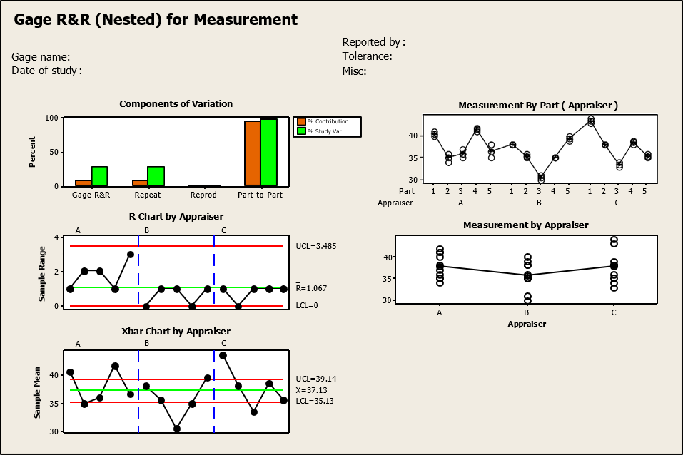
Next let's review the graphical output from Minitab's Gauge R&R (Nested) procedure.

These graphs are all part of a standard Gauge R&R analysis.

• The Components of Variation bar graph shows that the part‐to‐part variation is the largest component of both total process variation (variance of the dataset) and the study variation (using the sum of the Gauge R&R and part variation). This finding is consistent with a good measurement system.
• The Range (R) Chart by Appraiser plots the range of the measurements taken by each appraiser on each 'part.' It helps evaluate whether appraisers are consistent. For the measurement system to be acceptable, all points should fall within the control limits (the two red lines). Any out‐of‐control points or non‐random patterns should be investigated before proceeding — this could be a result of appraiser technique, position error or instrument inconsistency.

Our chart appears to be in control so we can move on...

• The Xbar ( X ) Chart by Appraiser shows the average of each appraiser's measurements on each 'part'. The area between the two control limits in this case represents the measurement system variation, so too many points falling inside this band means that the instrument is unable to distinguish between the parts. To be acceptable, approximately one‐half or more of the points should fall outside the limits on this graph. With 8 out of 15 points (53% — some of the points appearing on the outer edge of the line are actually outside it) falling outside the limits, our measurement system is able to detect part‐to‐part differences.
• The Measurement by Part (Appraiser) graph shows the individual measurements taken by appraiser A on all parts followed by those of appraisers B and C. This particular graph does not give much useful information on our study because the parts are not repeated across appraisers.
• The Measurement by Appraiser graph shows the individual readings for each appraiser. The line connecting the three sets of points represents the grand average of all readings for each appraiser. The flatter this line, the closer the averages. From this graph you can see that the line is quite flat, indicating that the three appraisers have similar averages. The spread of the points per appraiser shows that appraiser A's measurements have slightly lower variation than either appraiser B or C.

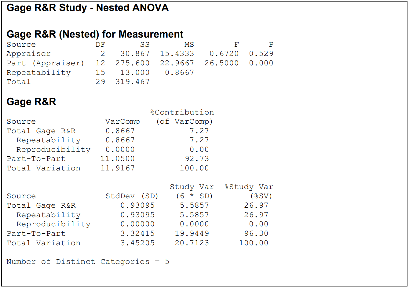
Finally let's look at the numbers — from the nested ANOVA summary output, also an important part of this study. This output is basically the same as (and is interpreted in the same way as) that of a standard GRR study, except that the parts are nested within appraisers, denoted as 'Part (Appraiser)' in the Anova table.

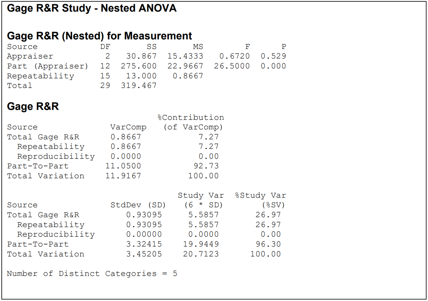
In the Anova table, any source factor with a p‐value (less than 5%) is considered to be a significant contributor to the total variation. Our ANOVA table supports the conclusions from the graphs — the large Appraiser p‐value (0.529) indicates that the contribution of the differences among appraisers to the total variation is not significant. The small p‐value for Parts shows that part‐to‐part variation is significant. The Number of Distinct Categories indicates the number of distinct data categories that the measurement system can discern within the sample. This number must be 5 or more for the measurement system to be acceptable for analysis — in our case it is exactly 5, so this is evidence that the system is able to correctly distinguish between the parts.

The acceptability of the gauge finally boils down to the percentage contribution of each source (Parts, Appraisers, Measurement system) to the total variation and to the study variation. Notice that the contribution of Reproducibility to the total variation is zero — this is because no two appraisers measured the same part. The Parts are the largest source (accounting for 93% of the total variation and 96.3% of the study variation), whereas Gauge R&R accounts for 7.3% of total variation and 27% of the study variation. A Gauge R&R component of 30% or less is generally considered acceptable, so our instrument appears to have made the grade.

Key Points to Consider

1. In any non‐replicable study such as this one, the Gauge RR percentage necessarily includes some process variation. Because different parts are used across trials, there is no way to separate all process variation from measurement system variation in this scheme.
2. This is a single event study. It may be used to initially qualify a system, but more work is required to control that measurement system over time to ensure its stability and usefulness in making the appropriate process control and/or capability decisions and continuous improvement. To keep tabs on this measurement process over time, a control chart could be used periodically to determine the system's stability.