The Use of Dummy Variables in Regression Analysis

What is a Dummy variable?

A Dummy variable or Indicator variable is an artificial variable created to represent a categorical variable with two or more distinct categories or levels.

Why is it used?

Regression analysis treats all independent (X) variables in the analysis as numerical. Numerical variables are interval or ratio scale variables whose values are directly comparable, for example, "3 minus 1 equals 2", or "10 is twice as much as 5". You might often want to include a categorical or nominal scale variable such as "Product Brand" or "Type of Defect" in your study. Say you have three types of defects, numbered "1", "2" and "3". In this case, "3 minus 1" implies you are subtracting defect "1" from defect "3", which doesn’t mean anything – the numbers here are simply used to identify the levels of "Defect Type" and do not have any intrinsic meaning on their own. Dummy variables are created in this situation to "trick" the regression algorithm into correctly analyzing attribute variables. Typically, the software will do this in the background so you dont have to do it in the front end.

How is a dummy variable created?

We will illustrate this with an example: Let's say you want to find out whether two categorical variables – the location of a house (in the East, SouthEast or NorthWest side of a development) and when the house was built (before, or after, 1990) – affect its sale price (the Y, or response variable.) The image below shows a portion of the Sale Price dataset:

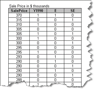
SalePrice is the numerical response variable. The binary variable Y1990 represents the independent (X) variable 'Before or After 1990' by taking on two values:

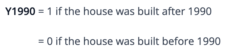
Y1990 becomes an indicator (dummy) variable representing the category to which a house belongs (before or after 1990.) Note that a single dummy variable is sufficient to represent a variable with two levels.

Next, we want to represent the location of the house among the three possible categories (E, SE, NW). The data set contains two binary variables: 'E' (East) and 'SE' (SouthEast). They're dummy variables, constructed such that:

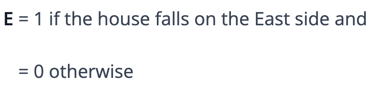
But what happens to the third location, NW? Well, it turns out we don’t need a third dummy variable to represent it; setting both 'E' and 'SE' dummy variables to '0' indicates a house that is neither on the East nor the SE side, so it must fall on the NW side. Notice that this coding only works if the three categories are mutually exclusive (do not overlap) and exhaustive (no other categories exist for this variable besides these three), at least as far as this analysis is concerned. Since NW does not itself appear as a dummy variable but is implied by setting both E and SE to '0', it is called the 'reference level.'

The regression of SalePrice on these dummy variables yields the following model:

The intercept value of 258, obtained by setting each of the terms (Y1990, E, and SE) to '0', indicates that the average price of a house built before 1990 on the NW side of this neighborhood is $258K. The coefficient of Y1990 is 33.9, indicating that all other things being equal, houses in this neighborhood built after 1990 command a $33.9K premium over those built before 1990. Note, here 'built before 1990', the condition where Y1990 takes the value '0', is the 'reference level.'

Moving on to the next coefficient, houses on the East side cost, on average, $10.7K lower (given its negative sign) than houses on the NW side; similarly, houses on the SE side cost, on average, $21K higher than houses on the NW side. Thus, NW is the ‘reference’ or ‘comparison’ level for E and SE.

You can estimate the sale price for a house built before 1990 and located on the East side from this equation by substituting Y1990 = 0, E = 1, and SE = 0, giving the SalePrice = $247.3K.

Things to keep in mind about dummy variables

Dummy variables assign the numbers '0' and '1' to indicate membership in any mutually exclusive and exhaustive category.

1. The number of dummy variables necessary to represent the levels of a single attribute variable is equal to the number of levels (categories) in that variable, minus one.
2. None of the dummy variables constructed can be redundant for a given attribute variable. That is, one dummy variable can't be a constant multiple or a simple linear relation of another.
3. The interaction of two attribute variables (e.g., Smoking and Heart Disease) is represented by a third dummy variable which is simply the product of the two individual dummy variables.
4. The interaction of two numeric variables with an attribute variable (e.g., Age and Heart Disease) is represented by the product of the numeric and the dummy variables.

As you have seen, creating indicator or dummy variables is a very useful concept and makes it possible to include categorical variables in a regression analysis.